Purpose: visualize long-term population estimate, redd count, and spawning weir data from multiple YCT populations in the upper Snake River watershed.
2.1 Data
Code
# mark-recapture population estimatespopest <-read_csv("C:/Users/jbaldock/OneDrive - DOI/Documents/WyACT/Snake River Assessment/Population data/PopulationEstimates_WGFD_1988-2022_cleaned.csv") %>%mutate(Nperkm_total = Npermile_total/1.60934)# spring creek redd countsreddcts <-read_csv("C:/Users/jbaldock/OneDrive - DOI/Documents/WyACT/Snake River Assessment/Population data/ReddCounts_WGFD_1971-2021_cleaned.csv")# lower bar bc weir (latent run size following run timing model)weir <-read_csv("C:/Users/jbaldock/OneDrive - DOI/Documents/WyACT/Snake River Assessment/Population data/RunTiming_TopModel_MalFem2_ParameterSummary.csv")names(weir) <-c("param", "mean", "sd", "ci025", "ci_250", "ci_500", "ci_750", "ci_975", "Rhat", "n.eff")weirtib <-tibble(year =rep(NA, times =55),param =rep(NA, times =55),total_mean =rep(NA, times =55),total_sd =rep(NA, times =55))weirtib$year <-c(1965:1990, 1992:2015, 2017:2021)for (i in1:55) { weirtib$param[i] <-unlist(weir[i+174,1]) # parameter name weirtib$total_mean[i] <-unlist(weir[i+174,2]) # mean total run size weirtib$total_sd[i] <-unlist(weir[i+174,3]) # SD total run size}
2.2 Mark-Recapture
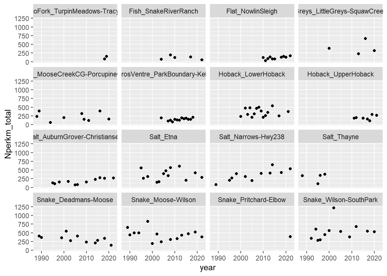
View all data:
Code
popest %>%ggplot(aes(x = year, y = Nperkm_total)) +geom_point() +#geom_line() +facet_wrap(~site)
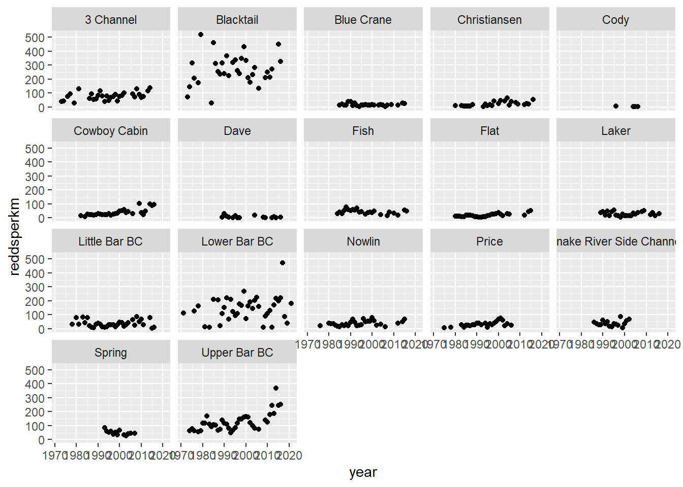
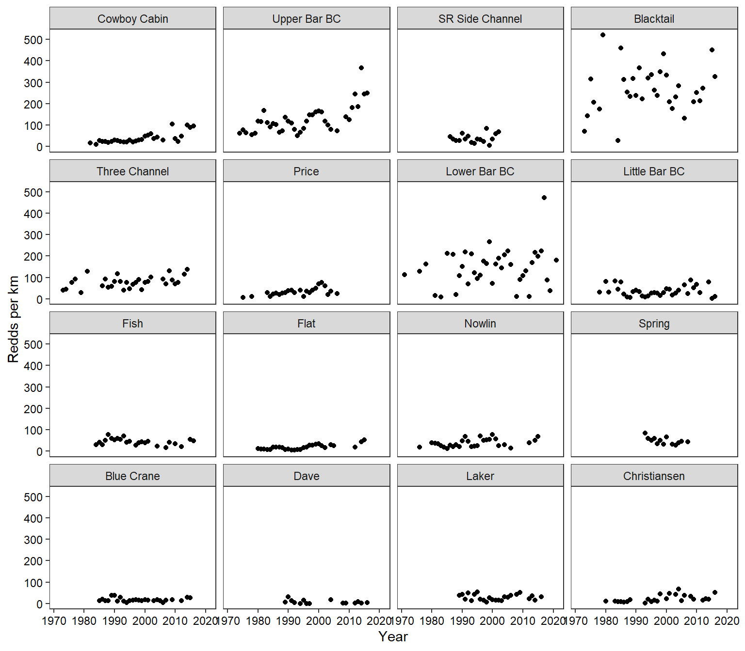
reddcts %>%ggplot(aes(x = year, y = reddsperkm)) +geom_point() +facet_wrap(~stream)
Drop Cody Creek (only 4 years or data) and fix names
Code
reddcts %>%filter(stream !="Cody") %>%mutate(stream =recode(stream, "3 Channel"="Three Channel", "Snake River Side Channel"="SR Side Channel")) %>%mutate(stream =factor(stream, levels =c("Cowboy Cabin", "Upper Bar BC", "SR Side Channel", "Blacktail","Three Channel", "Price", "Lower Bar BC", "Little Bar BC", "Fish", "Flat", "Nowlin", "Spring", "Blue Crane", "Dave", "Laker", "Christiansen"))) %>%ggplot(aes(x = year, y = reddsperkm)) +#geom_smooth() +geom_point() +facet_wrap(~stream) +xlab("Year") +ylab("Redds per km") +#ylim(0,900) +theme_bw() +theme(panel.grid =element_blank(), axis.text =element_text(color ="black"))
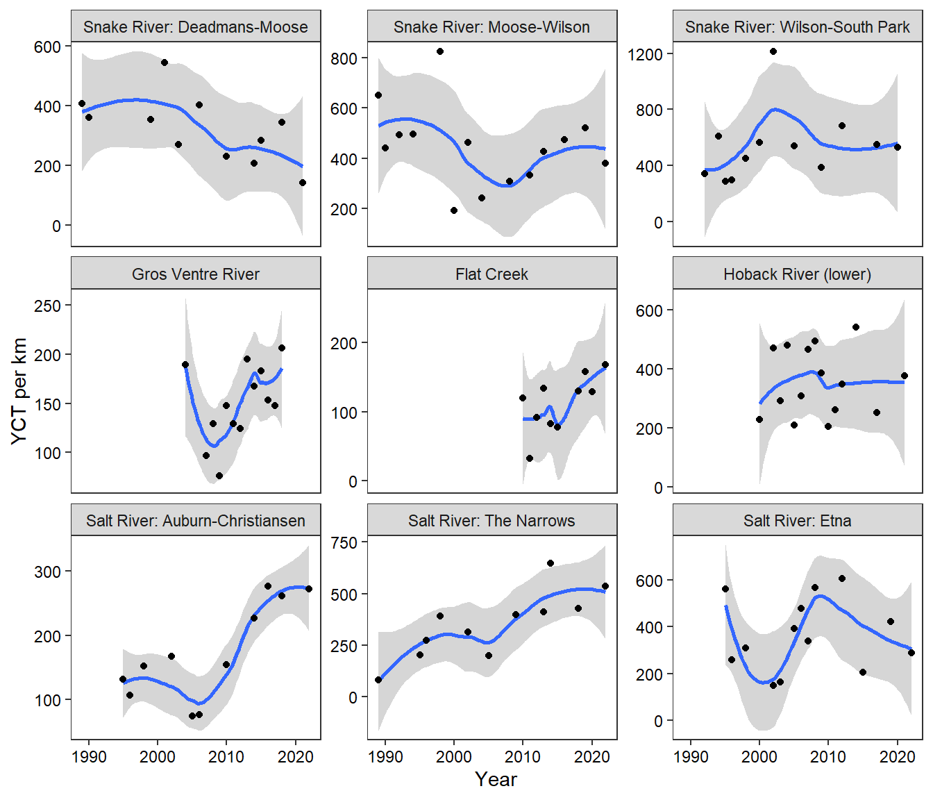
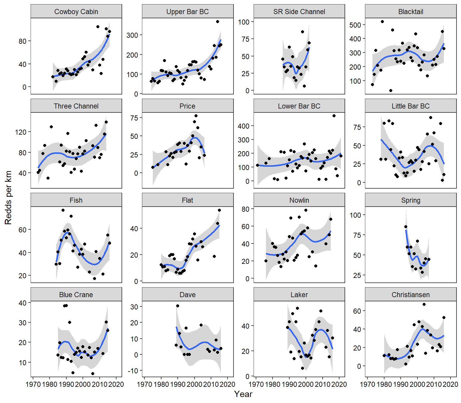
Add LOESS smoothers and plot on unique scales:
Code
reddcts %>%filter(stream !="Cody") %>%mutate(stream =recode(stream, "3 Channel"="Three Channel", "Snake River Side Channel"="SR Side Channel")) %>%mutate(stream =factor(stream, levels =c("Cowboy Cabin", "Upper Bar BC", "SR Side Channel", "Blacktail","Three Channel", "Price", "Lower Bar BC", "Little Bar BC", "Fish", "Flat", "Nowlin", "Spring", "Blue Crane", "Dave", "Laker", "Christiansen"))) %>%ggplot(aes(x = year, y = reddsperkm)) +geom_smooth() +geom_point() +facet_wrap(~stream, scales ="free_y") +xlab("Year") +ylab("Redds per km") +#ylim(0,900) +theme_bw() +theme(panel.grid =element_blank(), axis.text =element_text(color ="black"))
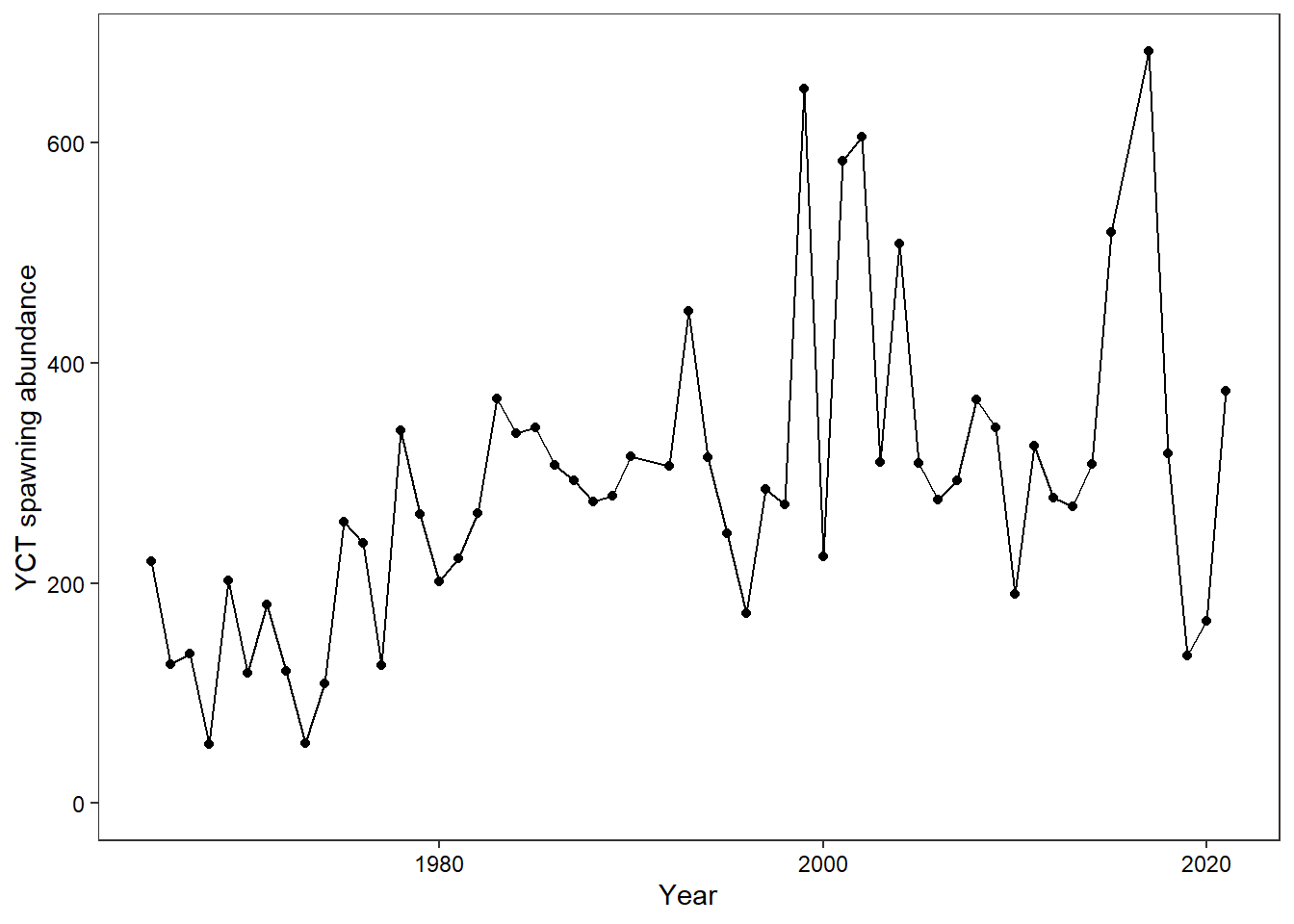
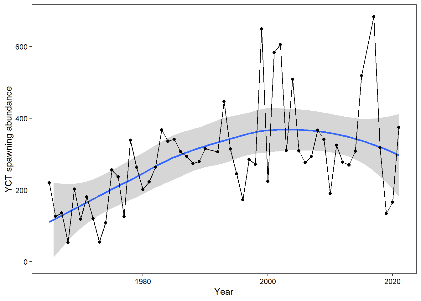
2.4 Weir
Plot time series of YCT spawning abundance in Lower Bar BC (enumerated at the WGFD weir). Abundance data are corrected for interannual variation in monitoring period using a run timing model as in Baldock et al. (2023, CJFAS).