dat <-read_csv("data/EcoDrought_FlowTempData_DailyWeekly_clean.csv")dat
# A tibble: 167,535 × 23
   site_name  basin date       flow_mean tempc_mean tempc_min tempc_max Yield_mm
   <chr>      <chr> <date>         <dbl>      <dbl>     <dbl>     <dbl>    <dbl>
 1 Avery Bro… <NA>  2020-01-01     NA       NA         NA        NA        NA
 2 Avery Bro… <NA>  2020-01-02     NA       NA         NA        NA        NA
 3 Avery Bro… <NA>  2020-01-03     NA       NA         NA        NA        NA
 4 Avery Bro… <NA>  2020-01-04     NA       NA         NA        NA        NA
 5 Avery Bro… <NA>  2020-01-05     NA       NA         NA        NA        NA
 6 Avery Bro… <NA>  2020-01-06     NA       NA         NA        NA        NA
 7 Avery Bro… <NA>  2020-01-07     NA       NA         NA        NA        NA
 8 Avery Bro… West… 2020-01-08      5.96     0.594      0.111     1.11      1.99
 9 Avery Bro… West… 2020-01-09      4.81     0.0336     0         0.111     1.61
10 Avery Bro… West… 2020-01-10      4.88     0.363      0         0.778     1.63
# ℹ 167,525 more rows
# ℹ 15 more variables: lat <dbl>, long <dbl>, area_sqmi <dbl>, elev_ft <dbl>,
#   yday <dbl>, air_temp_mean <dbl>, precip_mmday <dbl>, swe_kgm2 <dbl>,
#   daylength_sec <dbl>, shortrad_wm2 <dbl>, index <dbl>, year <dbl>,
#   count <dbl>, siteYear <chr>, movingMean <dbl>
Fix basins and trim to focal variables.
Code
mysitebasins <- dat %>%group_by(site_name) %>%summarize(basin =unique(basin),lat =unique(lat), long =unique(long), elev_ft =unique(elev_ft),area_sqmi =unique(area_sqmi)) %>%filter(!is.na(basin), !is.na(lat), !is.na(long), !is.na(elev_ft), !is.na(area_sqmi)) %>%mutate(basin =recode(basin, "Shields River"="Yellowstone"))dat <- dat %>%select(-c(basin, lat, long, elev_ft, area_sqmi)) %>%left_join(mysitebasins) %>%select(site_name, basin, lat, long, elev_ft, area_sqmi, date, yday, year, siteYear, tempc_mean, tempc_min, tempc_max, flow_mean, Yield_mm, air_temp_mean, precip_mmday, swe_kgm2, daylength_sec, shortrad_wm2)dat
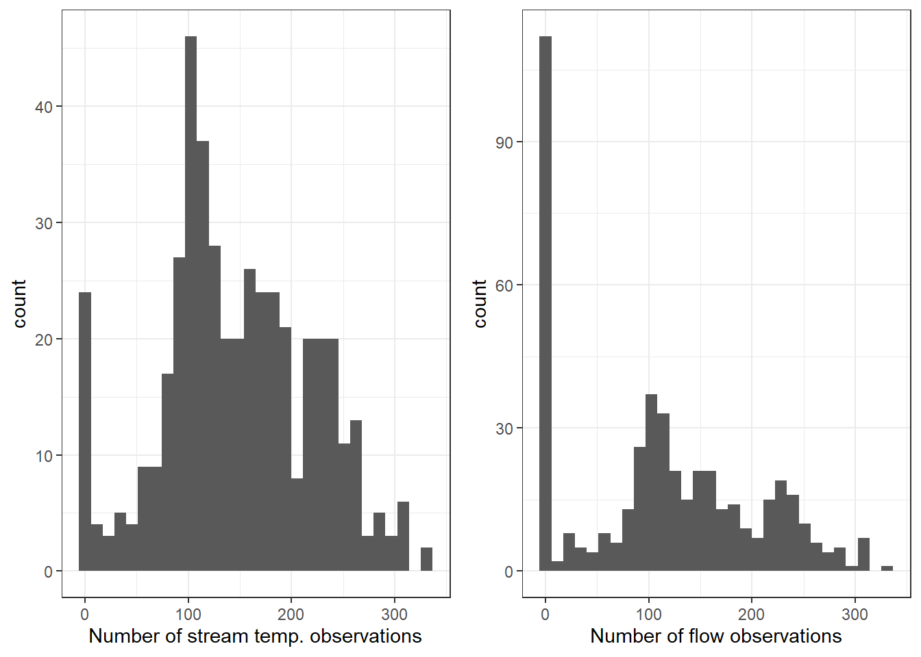
Show the distribution of the number of stream temp/flow observations (non-NA) per site-year…many years with poor data coverage, especially with respect to flow
Z-score air temp, flow, and day of year. Note: variables are standardized both by site (“z_…”) and by basin (“zbas_…”).
Code
# calculate lagged air tempdat_bp <- dat_bp %>%group_by(site_name) %>%mutate(z_Yield_mm_log =c(scale(Yield_mm_log, center =TRUE, scale =TRUE)),z_air_temp_mean =c(scale(air_temp_mean, center =TRUE, scale =TRUE)),z_air_temp_mean_lag1 =c(scale(air_temp_mean_lag1, center =TRUE, scale =TRUE)), #lag(z_air_temp_mean, n = 1),z_air_temp_mean_lag2 =c(scale(air_temp_mean_lag2, center =TRUE, scale =TRUE)) #lag(z_air_temp_mean, n = 2),#z_yday = c(scale(yday, center = TRUE, scale = TRUE)) ) %>%ungroup() %>%group_by(basin) %>%mutate(zbas_Yield_mm_log =c(scale(Yield_mm_log, center =TRUE, scale =TRUE)),zbas_air_temp_mean =c(scale(air_temp_mean, center =TRUE, scale =TRUE)),zbas_air_temp_mean_lag1 =c(scale(air_temp_mean_lag1, center =TRUE, scale =TRUE)), #lag(zbas_air_temp_mean, n = 1),zbas_air_temp_mean_lag2 =c(scale(air_temp_mean_lag2, center =TRUE, scale =TRUE)) #lag(zbas_air_temp_mean, n = 2),#zbas_yday = c(scale(yday, center = TRUE, scale = TRUE)) ) %>%ungroup()
Create dummy site and basin variables (numeric for JAGS), and define “rowNum” variable to allow for identifying first rows and evaluation rows
Code
# # Drop sites without any flow or water temp observations# dropsites <- unlist(dat_bp %>% # group_by(site_name) %>% # summarize(numt = sum(!is.na(tempc_mean)), # numf = sum(!is.na(z_Yield_mm_log))) %>% # ungroup() %>%# filter(numt == 0 | numf == 0) %>%# select(site_name))# dat_bp <- dat_bp %>% filter(!site_name %in% dropsites)# arrangedat_bp <- dat_bp %>%arrange(basin, site_name, year, yday)# create tibbles of site and basin numeric codessitecodes <-tibble(site_name =unique(dat_bp$site_name), site_code =1:length(unique(dat_bp$site_name)))basincodes <-tibble(basin =unique(dat_bp$basin), basin_code =1:length(unique(dat_bp$basin)))# join to data and define row numberdat_bp <- dat_bp %>%left_join(sitecodes) %>%left_join(basincodes) %>%mutate(rowNum =1:nrow(.))
4.2 Landscape covariates
To do – derive additional landscape covariates presumed to affect stream temperature, or rather, mediate the relationship between stream and air temperature/flow (groundwater influence/pasta?, basin slope, lake area, percent forest cover, etc.)
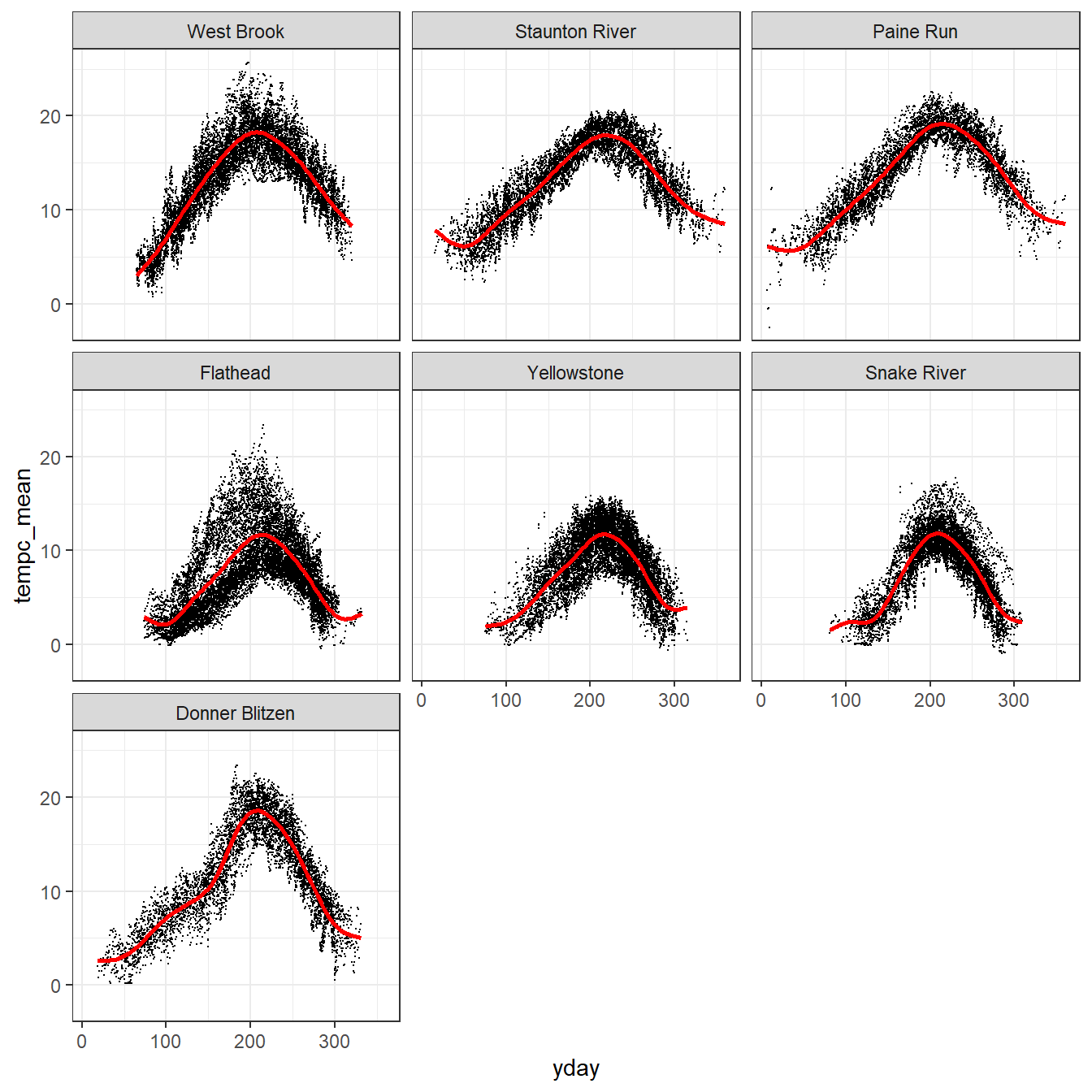
---title: "Format Data"---**Purpose:** Format data for modeling in JAGS```{r include=FALSE}library(ggplot2)library(tidyverse)#library(nlme)# library(devtools)# #install_github("conteStreamTemperature", username = "Conte-Ecology")# library(conteStreamTemperature)```## Base dataTemperature and flow data```{r}dat <-read_csv("data/EcoDrought_FlowTempData_DailyWeekly_clean.csv")dat```Fix basins and trim to focal variables.```{r}mysitebasins <- dat %>%group_by(site_name) %>%summarize(basin =unique(basin),lat =unique(lat), long =unique(long), elev_ft =unique(elev_ft),area_sqmi =unique(area_sqmi)) %>%filter(!is.na(basin), !is.na(lat), !is.na(long), !is.na(elev_ft), !is.na(area_sqmi)) %>%mutate(basin =recode(basin, "Shields River"="Yellowstone"))dat <- dat %>%select(-c(basin, lat, long, elev_ft, area_sqmi)) %>%left_join(mysitebasins) %>%select(site_name, basin, lat, long, elev_ft, area_sqmi, date, yday, year, siteYear, tempc_mean, tempc_min, tempc_max, flow_mean, Yield_mm, air_temp_mean, precip_mmday, swe_kgm2, daylength_sec, shortrad_wm2)dat```Calculate lagged air temp variables, logged flow variables, and daily change in SWE.```{r}# ensure proper orderingdat <- dat[order(dat$site_name, dat$year, dat$yday),]# calculate lagged air tempdat <- dat %>%mutate(Yield_mm_log =log(Yield_mm +0.00001),flow_mean_log =log(flow_mean +0.00001)) %>%group_by(site_name) %>%mutate(air_temp_mean_lag1 =lag(air_temp_mean, 1),air_temp_mean_lag2 =lag(air_temp_mean, 2),delta_swe = swe_kgm2 -lag(swe_kgm2, 1)) %>%ungroup()```### Trim to synchronized periodLoad breakpoints```{r}springFallBPs <-read_csv("data/breakpoints.csv") %>%mutate(basin =recode(basin, "Shields River"="Yellowstone"))springFallBPs```Join temp/flow data with breakpoints and filter to days within synchronized period.```{r}dat_bp <- dat %>%left_join(springFallBPs) %>%filter(yday >= finalSpringBP & yday <= finalFallBP)dat_bp```### Drop missing dataShow the distribution of the number of stream temp/flow observations (non-NA) per site-year...*many years with poor data coverage, especially with respect to flow*```{r}obspersy <- dat_bp %>%group_by(siteYear) %>%summarize(streamtemp_numobs =sum(!is.na(tempc_mean)),flow_numobs =sum(!is.na(Yield_mm))) %>%ungroup()paste(dim(obspersy)[1], " total site-years", sep ="")ggpubr::ggarrange(obspersy %>%ggplot() +geom_histogram(aes(x = streamtemp_numobs)) +theme_bw() +xlab("Number of stream temp. observations"), obspersy %>%ggplot() +geom_histogram(aes(x = flow_numobs)) +theme_bw() +xlab("Number of flow observations"), nrow =1)```Drop siteYears with less than 50 days of stream temp./flow observations```{r}drops <- obspersy %>%filter(streamtemp_numobs <50| flow_numobs <50)paste(dim(obspersy)[1]-dim(drops)[1], " filtered site-years", sep ="")dat_bp <- dat_bp %>%filter(!siteYear %in% drops$siteYear)```Now drop days with missing stream temperature data```{r}dat_bp <- dat_bp %>%filter(!is.na(tempc_mean))```### Show dataPlot temp data with LOESS to show seasonal hysteresis```{r fig.width=7, fig.height=7}dat_bp %>%ggplot(aes(x = yday, y = tempc_mean)) +geom_point(size =0.1) +facet_wrap(~factor(basin, levels =c("West Brook", "Staunton River", "Paine Run", "Flathead", "Yellowstone", "Snake River", "Donner Blitzen"))) +geom_smooth(color ="red", se =FALSE) +theme_bw() #+ theme(panel.grid = element_blank())```### Z-scores and dummy vars.Z-score air temp, flow, and day of year. *Note: variables are standardized both by site ("z_...") and by basin ("zbas_...").*```{r}# calculate lagged air tempdat_bp <- dat_bp %>%group_by(site_name) %>%mutate(z_Yield_mm_log =c(scale(Yield_mm_log, center =TRUE, scale =TRUE)),z_air_temp_mean =c(scale(air_temp_mean, center =TRUE, scale =TRUE)),z_air_temp_mean_lag1 =c(scale(air_temp_mean_lag1, center =TRUE, scale =TRUE)), #lag(z_air_temp_mean, n = 1),z_air_temp_mean_lag2 =c(scale(air_temp_mean_lag2, center =TRUE, scale =TRUE)) #lag(z_air_temp_mean, n = 2),#z_yday = c(scale(yday, center = TRUE, scale = TRUE)) ) %>%ungroup() %>%group_by(basin) %>%mutate(zbas_Yield_mm_log =c(scale(Yield_mm_log, center =TRUE, scale =TRUE)),zbas_air_temp_mean =c(scale(air_temp_mean, center =TRUE, scale =TRUE)),zbas_air_temp_mean_lag1 =c(scale(air_temp_mean_lag1, center =TRUE, scale =TRUE)), #lag(zbas_air_temp_mean, n = 1),zbas_air_temp_mean_lag2 =c(scale(air_temp_mean_lag2, center =TRUE, scale =TRUE)) #lag(zbas_air_temp_mean, n = 2),#zbas_yday = c(scale(yday, center = TRUE, scale = TRUE)) ) %>%ungroup()```Create dummy site and basin variables (numeric for JAGS), and define "rowNum" variable to allow for identifying first rows and evaluation rows```{r}# # Drop sites without any flow or water temp observations# dropsites <- unlist(dat_bp %>% # group_by(site_name) %>% # summarize(numt = sum(!is.na(tempc_mean)), # numf = sum(!is.na(z_Yield_mm_log))) %>% # ungroup() %>%# filter(numt == 0 | numf == 0) %>%# select(site_name))# dat_bp <- dat_bp %>% filter(!site_name %in% dropsites)# arrangedat_bp <- dat_bp %>%arrange(basin, site_name, year, yday)# create tibbles of site and basin numeric codessitecodes <-tibble(site_name =unique(dat_bp$site_name), site_code =1:length(unique(dat_bp$site_name)))basincodes <-tibble(basin =unique(dat_bp$basin), basin_code =1:length(unique(dat_bp$basin)))# join to data and define row numberdat_bp <- dat_bp %>%left_join(sitecodes) %>%left_join(basincodes) %>%mutate(rowNum =1:nrow(.))```## Landscape covariates*To do -- derive additional landscape covariates presumed to affect stream temperature, or rather, mediate the relationship between stream and air temperature/flow (groundwater influence/pasta?, basin slope, lake area, percent forest cover, etc.)*## Check correlations## Write to fileWrite formatted data to file```{r}write_csv(dat_bp, "data/EcoDrought_FlowTempData_formatted.csv")```