3 Snake model residuals

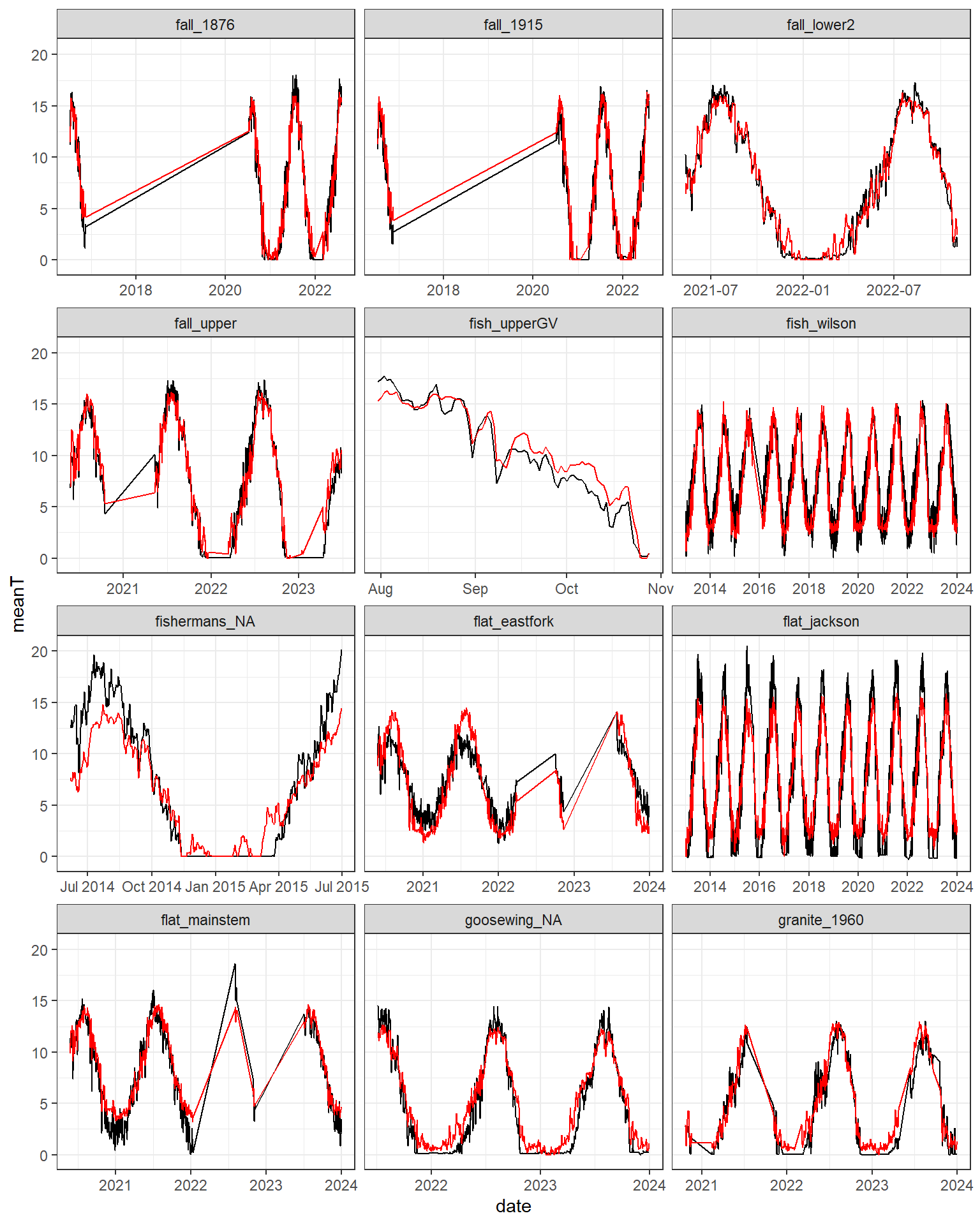
Purpose: Explore the relationship between residuals from K. Gauthier’s daily stream temperature model and independent metrics of groundwater availability. This is somewhat complicated by the fact that Kevin’s model already uses groundwater availability as a covariate, so we really aren’t evaluating how much additional information the groundwater metric adds, but rather the variance that isn’t explained by the existing metric (e.g., driven by spatial/temporal variation in groundwater temperature, lagged groundwater temperature signals, etc.).

3.1 Data

Load data from Kevin’s temp model:

Code

dat <- read_csv("Stream temperature/model_obs_pred_data.csv") %>% 
  mutate(model_resid = model_pred - meanT,
         year = as.factor(year(date))) %>%
  group_by(site, year) %>%
  mutate(model_resid_lag = lag(model_resid)) %>%
  ungroup()

head(dat)

# A tibble: 6 × 34
   ...1     X site        reachid  NEAR_X   NEAR_Y date         DOY dayl_rcamean
  <dbl> <dbl> <chr>         <dbl>   <dbl>    <dbl> <date>     <dbl>        <dbl>
1     1     1 bailey_1776     199 517826. 4784463. 2019-05-11   131         14.3
2     2     2 bailey_1776     199 517826. 4784463. 2019-05-12   132         14.4
3     3     3 bailey_1776     199 517826. 4784463. 2019-05-13   133         14.4
4     4     4 bailey_1776     199 517826. 4784463. 2019-05-14   134         14.4
5     5     5 bailey_1776     199 517826. 4784463. 2019-05-15   135         14.5
6     6     6 bailey_1776     199 517826. 4784463. 2019-05-16   136         14.5
# ℹ 25 more variables: h2oAreaKm2 <dbl>, h2oAreaKm2_log <dbl>,
#   h2oLakePerc <dbl>, forest_buff_perc <dbl>, h2o_slope_mean <dbl>,
#   h2o_streamslope_mean <dbl>, h2o_elev_mean <dbl>, logger_elev <dbl>,
#   elev_diff <dbl>, gw_influence <dbl>, prcp_rcamean <dbl>, prcp_3d <dbl>,
#   swe_rcamean <dbl>, swe_april1 <dbl>, airtemp_rcamean <dbl>,
#   airtemp_3d <dbl>, airtemp_5d <dbl>, airtemp_change_3d <dbl>,
#   airtemp_change_5d <dbl>, meanT <dbl>, model_pred <dbl>, …

Code

length(unique(dat$site))

[1] 78

3.2 Summarize error

“Global” RMSE

Code

sqrt(mean((dat$model_resid)^2))

[1] 1.422302

“Global” mean absolute error

Code

mean(abs(dat$model_resid))

[1] 1.087564

Plot relationships between model error (RMSE and MAE) and site-specific covariates

Code

errorterms <- dat %>%
  group_by(site) %>%
  summarize(gw_influence = mean(gw_influence),
            h2oAreaKm2_log = mean(h2oAreaKm2_log),
            forest_buff_perc = mean(forest_buff_perc),
            h2o_slope_mean = mean(h2o_slope_mean),
            h2o_elev_mean = mean(h2o_elev_mean),
            sampsize = n(),
            rmse = sqrt(mean((model_resid)^2)),
            mae = mean(abs(model_resid))) %>%
  ungroup()

# RMSE
p1 <- errorterms %>%
  ggplot(aes(x = log(gw_influence), y = rmse)) + 
  geom_point() +
  geom_smooth(method = "lm") +
  xlab("log(Groundwater influence)") + ylab("RMSE") +
  theme_bw() + theme(panel.grid = element_blank())

p2 <- errorterms %>%
  ggplot(aes(x = h2oAreaKm2_log, y = rmse)) + 
  geom_point() +
  geom_smooth(method = "lm") +
  xlab("log(Catchment area)") + ylab("RMSE") +
  theme_bw() + theme(panel.grid = element_blank())

p3 <- errorterms %>%
  ggplot(aes(x = forest_buff_perc, y = rmse)) + 
  geom_point() +
  geom_smooth(method = "lm") +
  xlab("Forest cover (% in buffer)") + ylab("RMSE") +
  theme_bw() + theme(panel.grid = element_blank())

p4 <- errorterms %>%
  ggplot(aes(x = h2o_slope_mean, y = rmse)) + 
  geom_point() +
  geom_smooth(method = "lm") +
  xlab("Mean catchment slope") + ylab("RMSE") +
  theme_bw() + theme(panel.grid = element_blank())

p5 <- errorterms %>%
  ggplot(aes(x = h2o_elev_mean, y = rmse)) + 
  geom_point() +
  geom_smooth(method = "lm") +
  xlab("Mean catchment elevation") + ylab("RMSE") +
  theme_bw() + theme(panel.grid = element_blank())

p6 <- errorterms %>%
  ggplot(aes(x = log(sampsize), y = rmse)) + 
  geom_point() +
  geom_smooth(method = "lm") +
  xlab("log(Sample size)") + ylab("RMSE") +
  theme_bw() + theme(panel.grid = element_blank())


# Mean Absolute Error
p1b <- errorterms %>%
  ggplot(aes(x = log(gw_influence), y = mae)) + 
  geom_point() +
  geom_smooth(method = "lm") +
  xlab("log(Groundwater influence)") + ylab("MAE") +
  theme_bw() + theme(panel.grid = element_blank())

p2b <- errorterms %>%
  ggplot(aes(x = h2oAreaKm2_log, y = mae)) + 
  geom_point() +
  geom_smooth(method = "lm") +
  xlab("log(Catchment area)") + ylab("MAE") +
  theme_bw() + theme(panel.grid = element_blank())

p3b <- errorterms %>%
  ggplot(aes(x = forest_buff_perc, y = mae)) + 
  geom_point() +
  geom_smooth(method = "lm") +
  xlab("Forest cover (% in buffer)") + ylab("MAE") +
  theme_bw() + theme(panel.grid = element_blank())

p4b <- errorterms %>%
  ggplot(aes(x = h2o_slope_mean, y = mae)) + 
  geom_point() +
  geom_smooth(method = "lm") +
  xlab("Mean catchment slope") + ylab("MAE") +
  theme_bw() + theme(panel.grid = element_blank())

p5b <- errorterms %>%
  ggplot(aes(x = h2o_elev_mean, y = mae)) + 
  geom_point() +
  geom_smooth(method = "lm") +
  xlab("Mean catchment elevation") + ylab("MAE") +
  theme_bw() + theme(panel.grid = element_blank())

p6b <- errorterms %>%
  ggplot(aes(x = log(sampsize), y = mae)) + 
  geom_point() +
  geom_smooth(method = "lm") +
  xlab("log(Sample size)") + ylab("MAE") +
  theme_bw() + theme(panel.grid = element_blank())

# combine plots
ggarrange(p1, p1b, 
          p2, p2b, 
          p3, p3b,
          p4, p4b,
          p5, p5b,
          p6, p6b, nrow = 6, ncol = 2, byrow = TRUE)

View pairs plots among site-specific covariates (some potential multicollinearity)

Code

ggpairs(errorterms %>% select(2:7))

Simple linear model quantifying the effect of site-specific covariates on model RMSE

Code

summary(lm(rmse ~ gw_influence + h2oAreaKm2_log + forest_buff_perc + h2o_slope_mean + h2o_elev_mean + sampsize, data = errorterms))


Call:
lm(formula = rmse ~ gw_influence + h2oAreaKm2_log + forest_buff_perc + 
    h2o_slope_mean + h2o_elev_mean + sampsize, data = errorterms)

Residuals:
     Min       1Q   Median       3Q      Max 
-0.65322 -0.24584 -0.06325  0.20642  1.18937 

Coefficients:
                   Estimate Std. Error t value Pr(>|t|)  
(Intercept)       1.052e+00  5.832e-01   1.803   0.0756 .
gw_influence      1.649e-01  3.020e-01   0.546   0.5867  
h2oAreaKm2_log   -9.849e-02  3.784e-02  -2.602   0.0113 *
forest_buff_perc -2.569e-03  2.193e-03  -1.171   0.2453  
h2o_slope_mean    7.075e-03  9.465e-03   0.748   0.4572  
h2o_elev_mean     3.271e-04  2.231e-04   1.466   0.1471  
sampsize         -4.748e-05  6.419e-05  -0.740   0.4619  
---
Signif. codes:  0 '***' 0.001 '**' 0.01 '*' 0.05 '.' 0.1 ' ' 1

Residual standard error: 0.379 on 71 degrees of freedom
Multiple R-squared:  0.1505,    Adjusted R-squared:  0.07876 
F-statistic: 2.097 on 6 and 71 DF,  p-value: 0.06417

3.3 Visualize residuals

3.3.1 Obs. and preds - scatter

Code

dat %>%
  ggplot(aes(x = meanT, y = model_pred)) +
  geom_point() +
  geom_abline(intercept = 0, slope = 1, color = "red") +
  theme_bw() + theme(panel.grid = element_blank()) +
  xlab("Observed temperature") + ylab("Predicted temperature")

Code

p <- dat %>%
  ggplot(aes(x = meanT, y = model_pred)) +
  geom_point(aes(color = year), alpha = 0.5) +
  geom_abline(intercept = 0, slope = 1, linetype = "dashed") +
  theme_bw() + theme(panel.grid = element_blank()) +
  xlab("Observed temperature") + ylab("Predicted temperature") +
  facet_wrap_paginate(~site, ncol = 3, nrow = 4, scales = "free_x")
n_pages(p)

[1] 7

Code

p + facet_wrap_paginate(~ site, ncol = 3, nrow = 4, page = 1)

Code

p + facet_wrap_paginate(~ site, ncol = 3, nrow = 4, page = 2)

Code

p + facet_wrap_paginate(~ site, ncol = 3, nrow = 4, page = 3)

Code

p + facet_wrap_paginate(~ site, ncol = 3, nrow = 4, page = 4)

Code

p + facet_wrap_paginate(~ site, ncol = 3, nrow = 4, page = 5)

Code

p + facet_wrap_paginate(~ site, ncol = 3, nrow = 4, page = 6)

Code

p + facet_wrap_paginate(~ site, ncol = 3, nrow = 4, page = 7)

3.3.2 Obs. and preds - time series

View time series with observations (black text) and model predictions (red text)

Code

p <- dat %>% 
  ggplot() +
  geom_line(aes(x = date, y = meanT)) + 
  geom_line(aes(x = date, y = model_pred), color = "red") +
  theme_bw() +
  facet_wrap_paginate(~site, ncol = 3, nrow = 4, scales = "free_x")
n_pages(p)

[1] 7

Code

p + facet_wrap_paginate(~ site, ncol = 3, nrow = 4, page = 1, scales = "free_x")

Code

p + facet_wrap_paginate(~ site, ncol = 3, nrow = 4, page = 2, scales = "free_x")

Code

p + facet_wrap_paginate(~ site, ncol = 3, nrow = 4, page = 3, scales = "free_x")

Code

p + facet_wrap_paginate(~ site, ncol = 3, nrow = 4, page = 4, scales = "free_x")

Code

p + facet_wrap_paginate(~ site, ncol = 3, nrow = 4, page = 5, scales = "free_x")

Code

p + facet_wrap_paginate(~ site, ncol = 3, nrow = 4, page = 6, scales = "free_x")

Code

p + facet_wrap_paginate(~ site, ncol = 3, nrow = 4, page = 7, scales = "free_x")

3.3.3 Residuals - time series

View all time series of residuals together

Code

dat %>%
  ggplot(aes(x = DOY, y = model_resid)) + 
  geom_point()

Facet by site, color by year:

Code

p <- dat %>% 
  ggplot() +
  geom_line(aes(x = DOY, y = model_resid, color = year)) +
  geom_abline(intercept = 0, slope = 0, linetype = "dashed") +
  theme_bw() +
  facet_wrap_paginate(~site, ncol = 3, nrow = 4)
n_pages(p)

[1] 7

Code

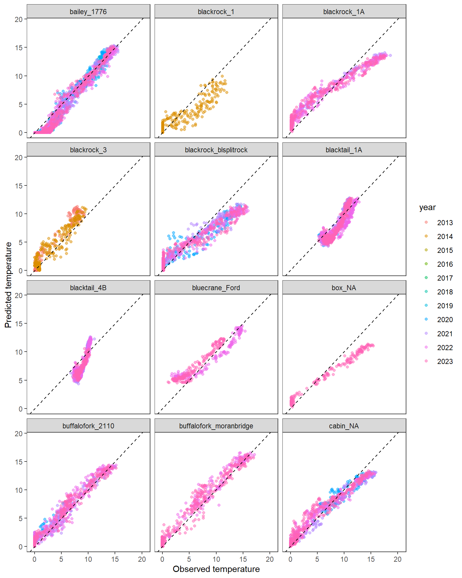
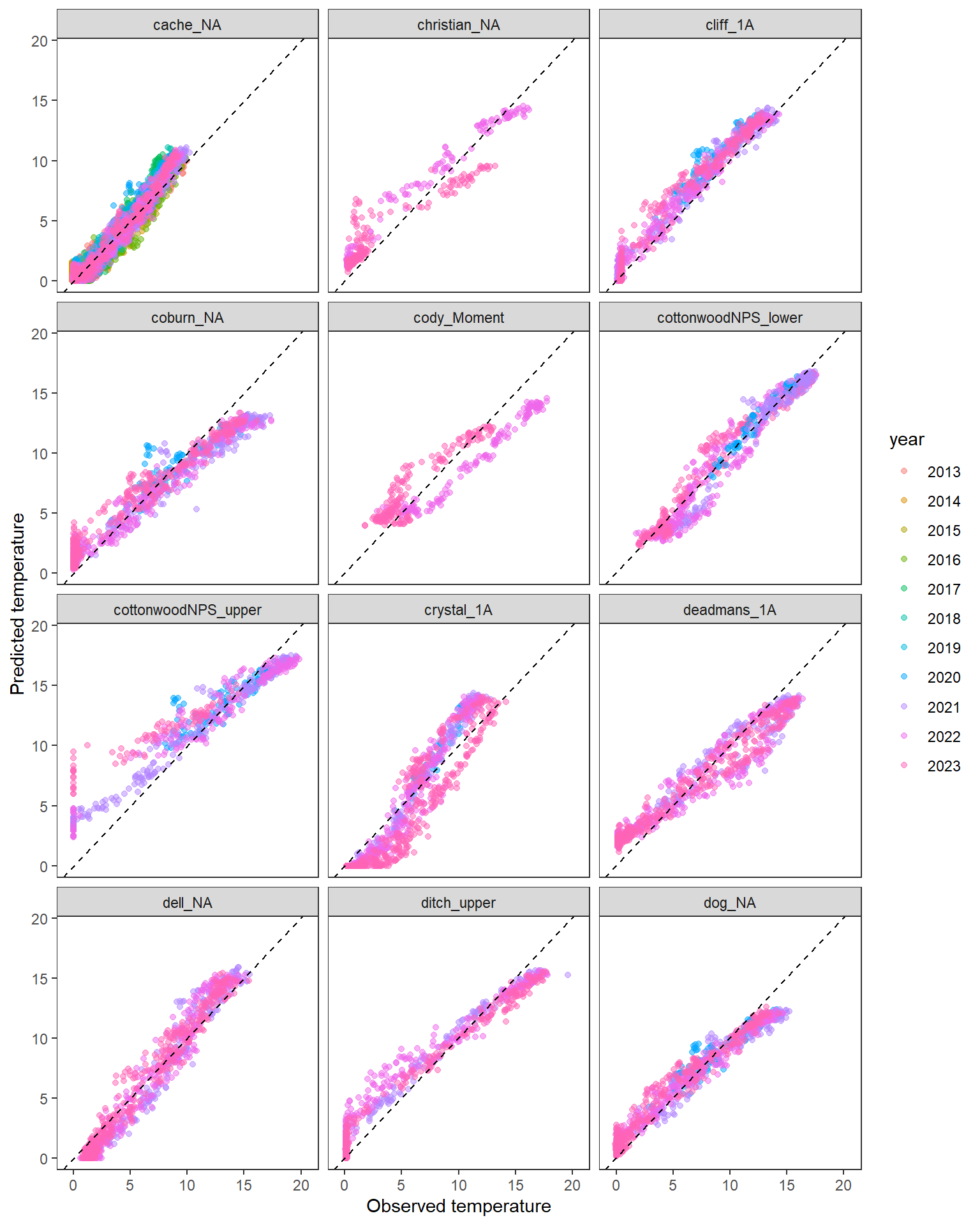
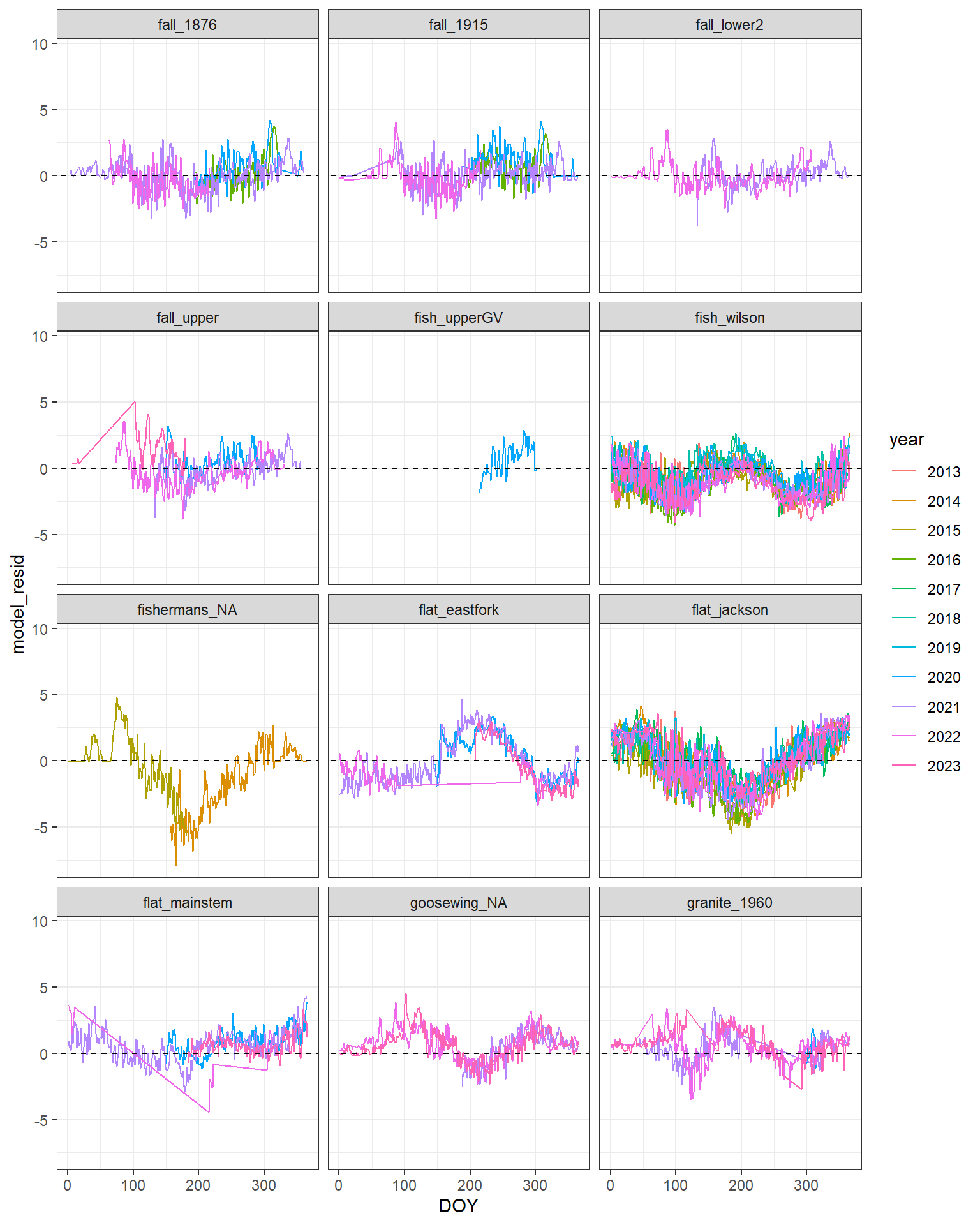
p + facet_wrap_paginate(~ site, ncol = 3, nrow = 4, page = 1)

Code

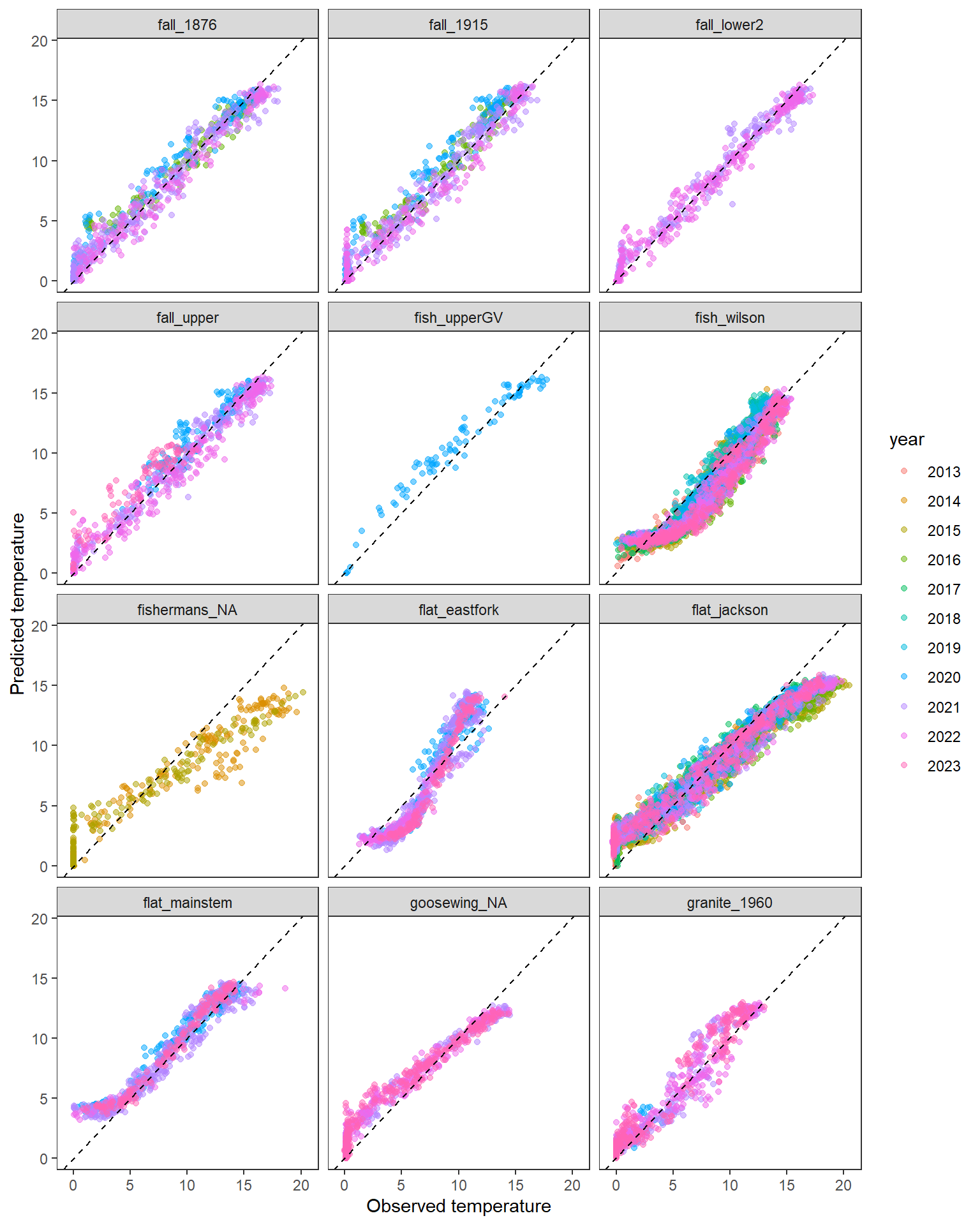
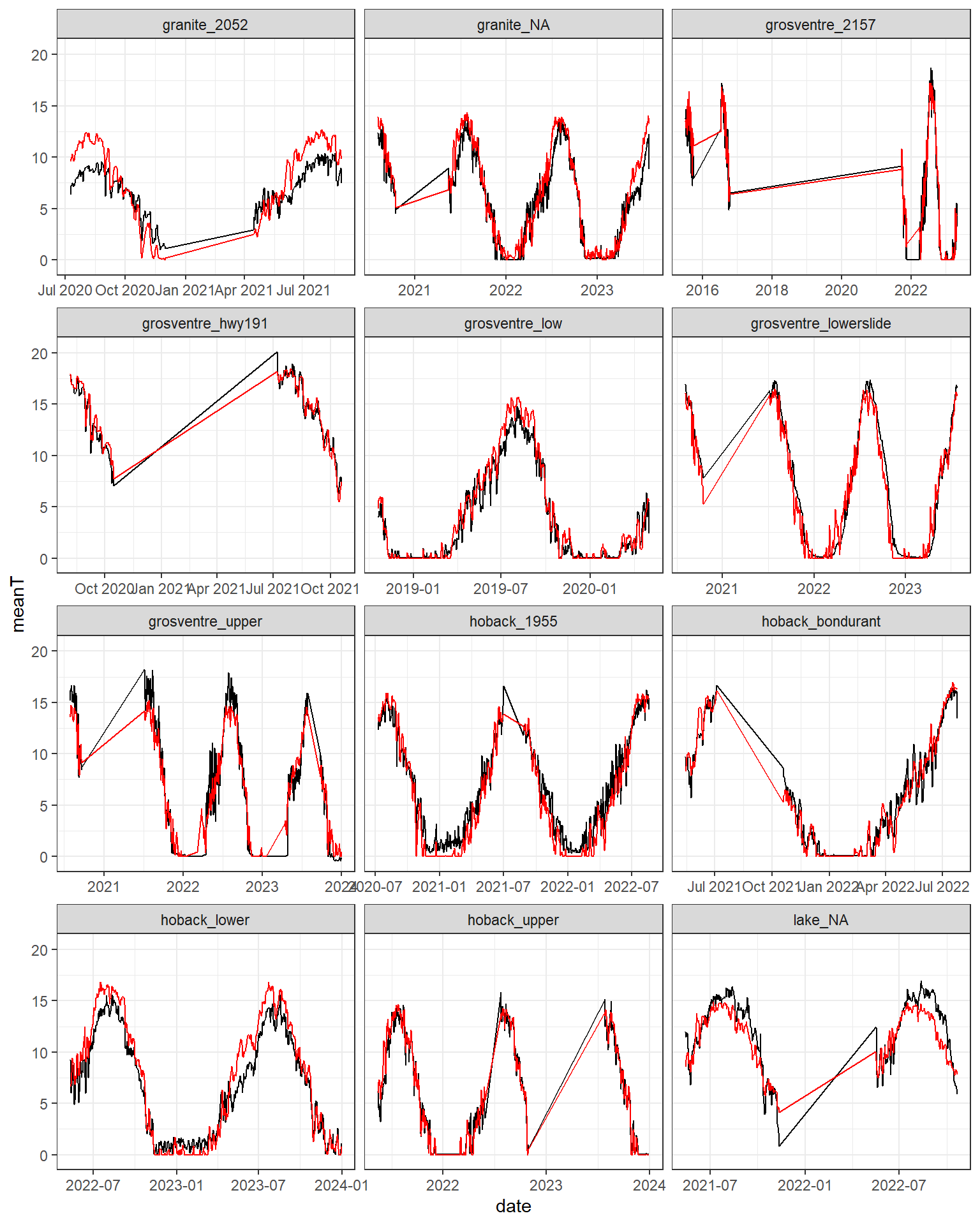
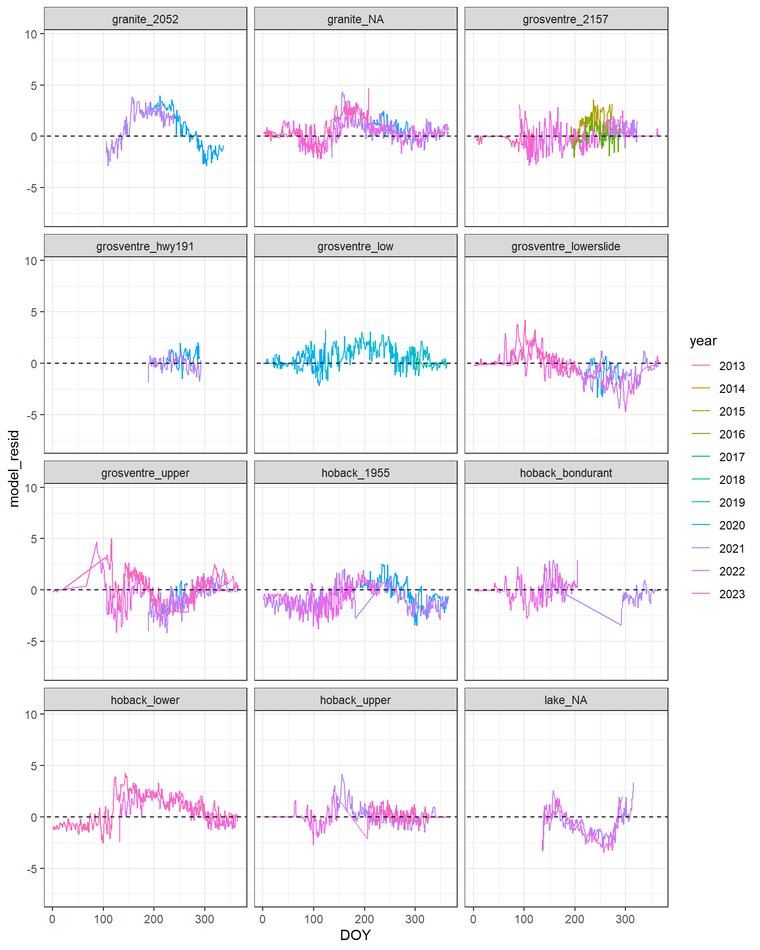
p + facet_wrap_paginate(~ site, ncol = 3, nrow = 4, page = 2)

Code

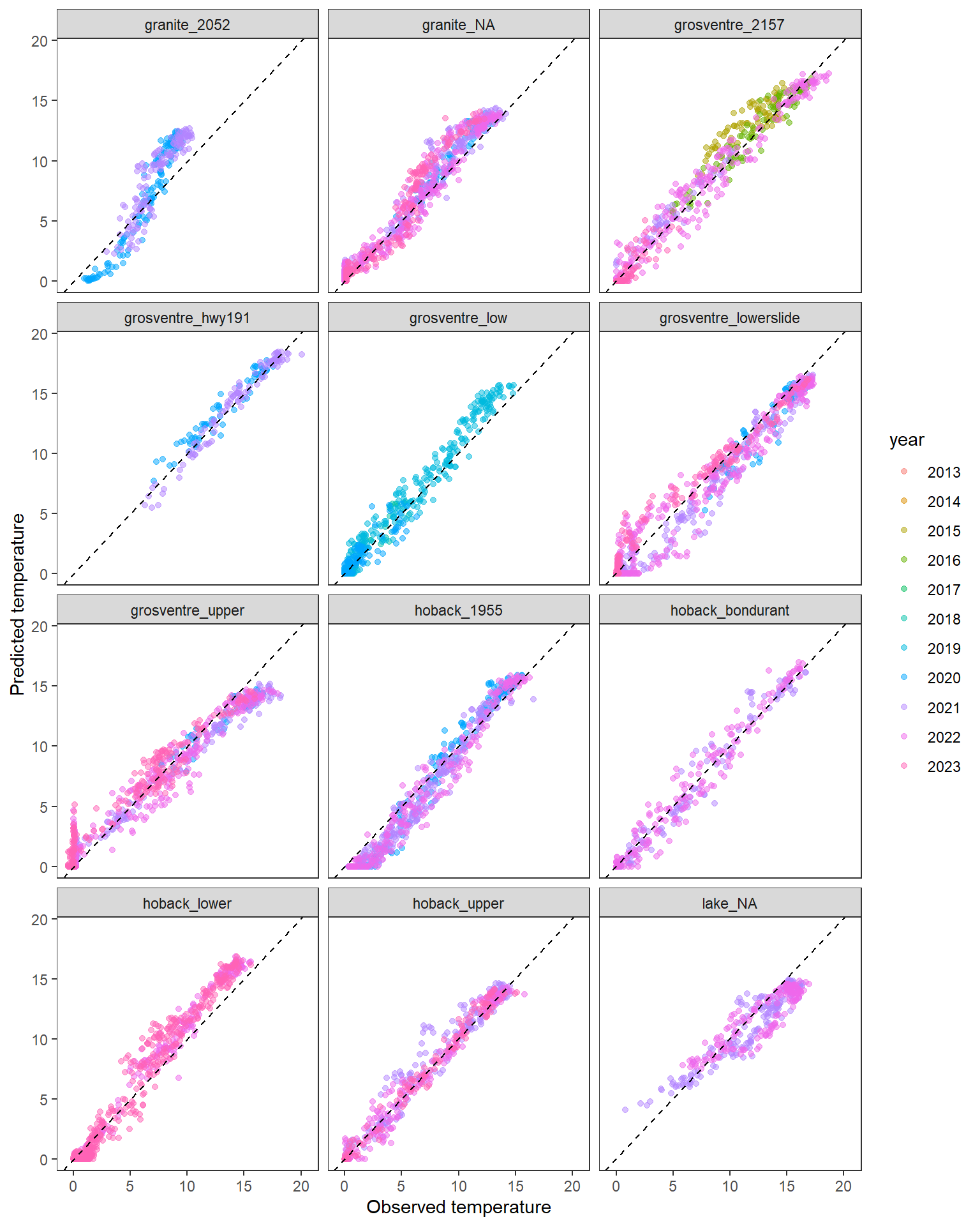
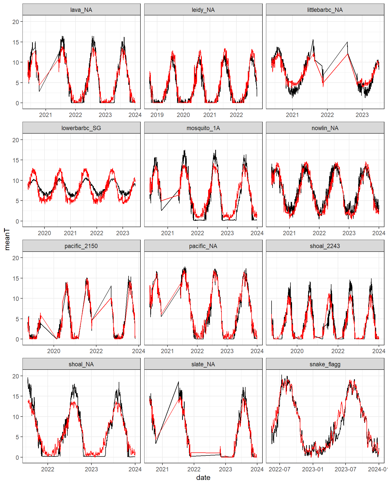
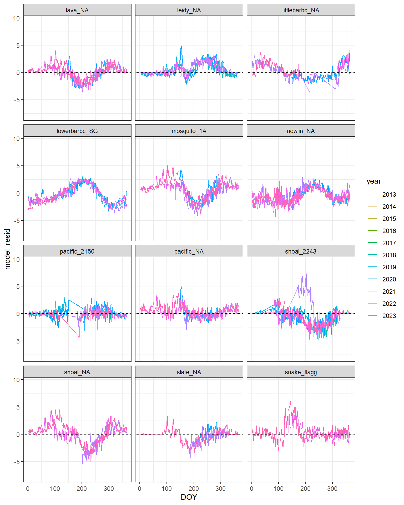
p + facet_wrap_paginate(~ site, ncol = 3, nrow = 4, page = 3)

Code

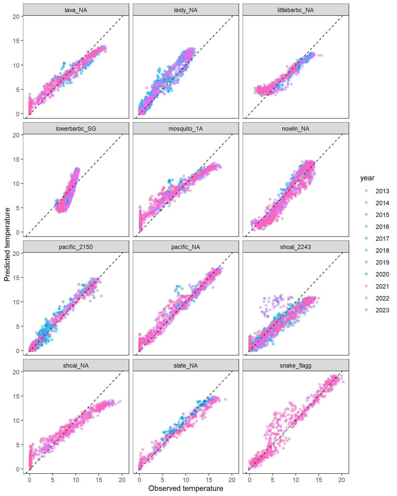
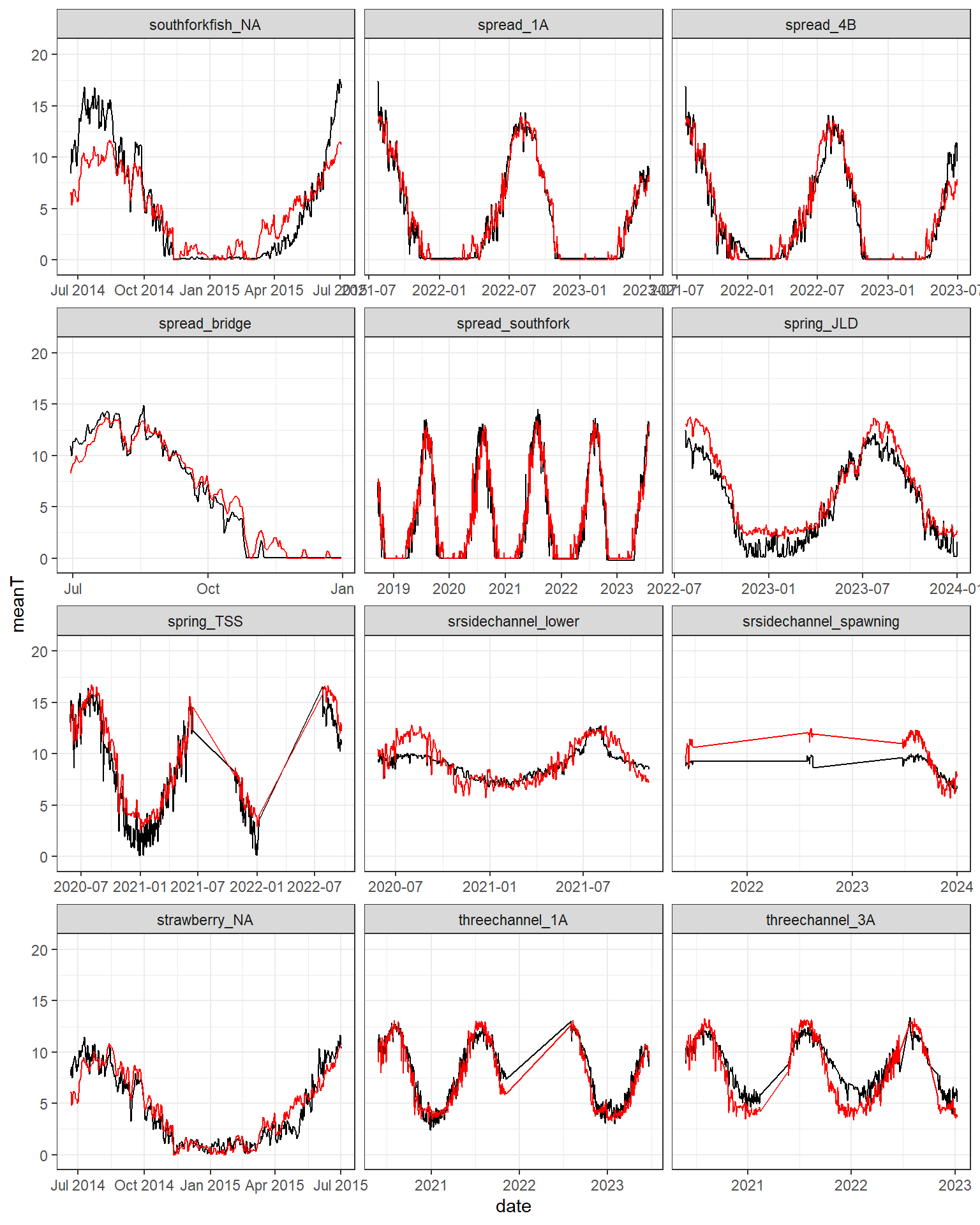
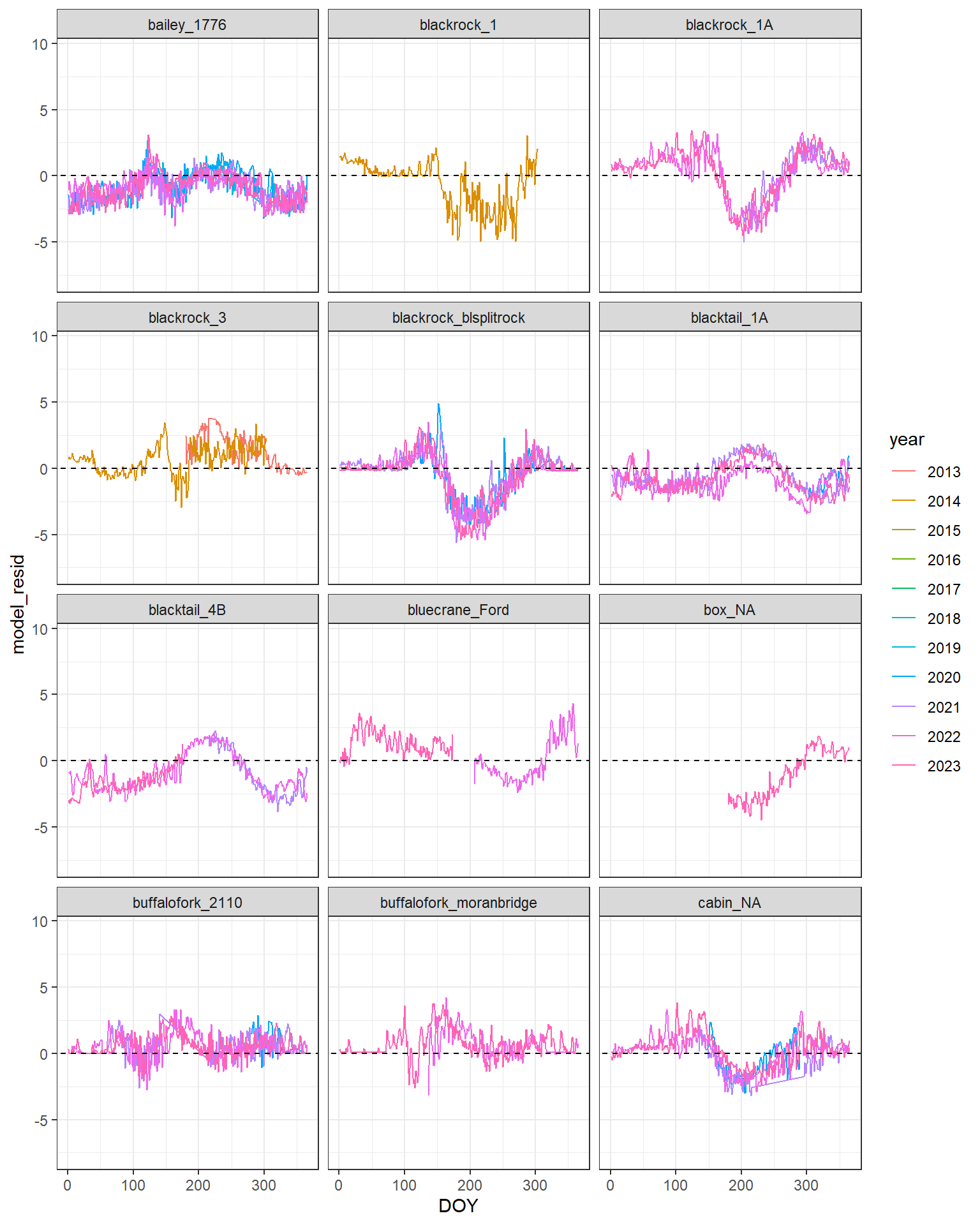
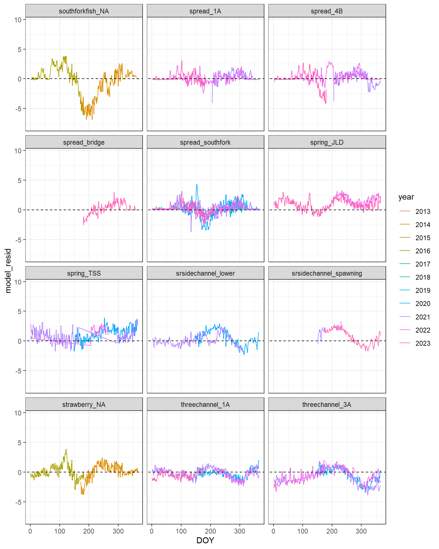
p + facet_wrap_paginate(~ site, ncol = 3, nrow = 4, page = 4)

Code

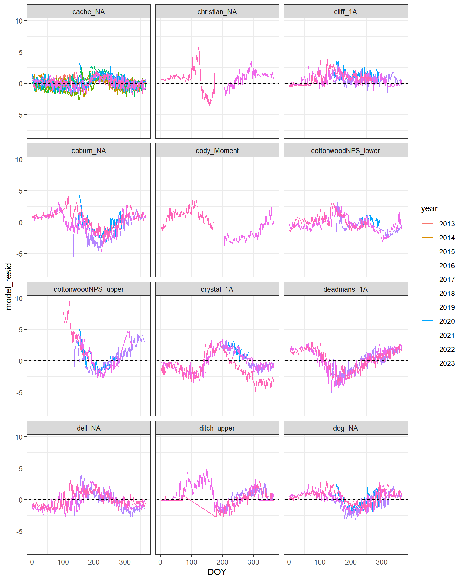
p + facet_wrap_paginate(~ site, ncol = 3, nrow = 4, page = 5)

Code

p + facet_wrap_paginate(~ site, ncol = 3, nrow = 4, page = 6)

Code

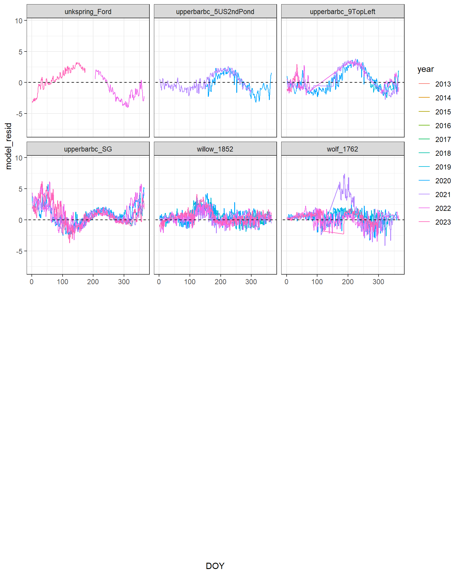
p + facet_wrap_paginate(~ site, ncol = 3, nrow = 4, page = 7)

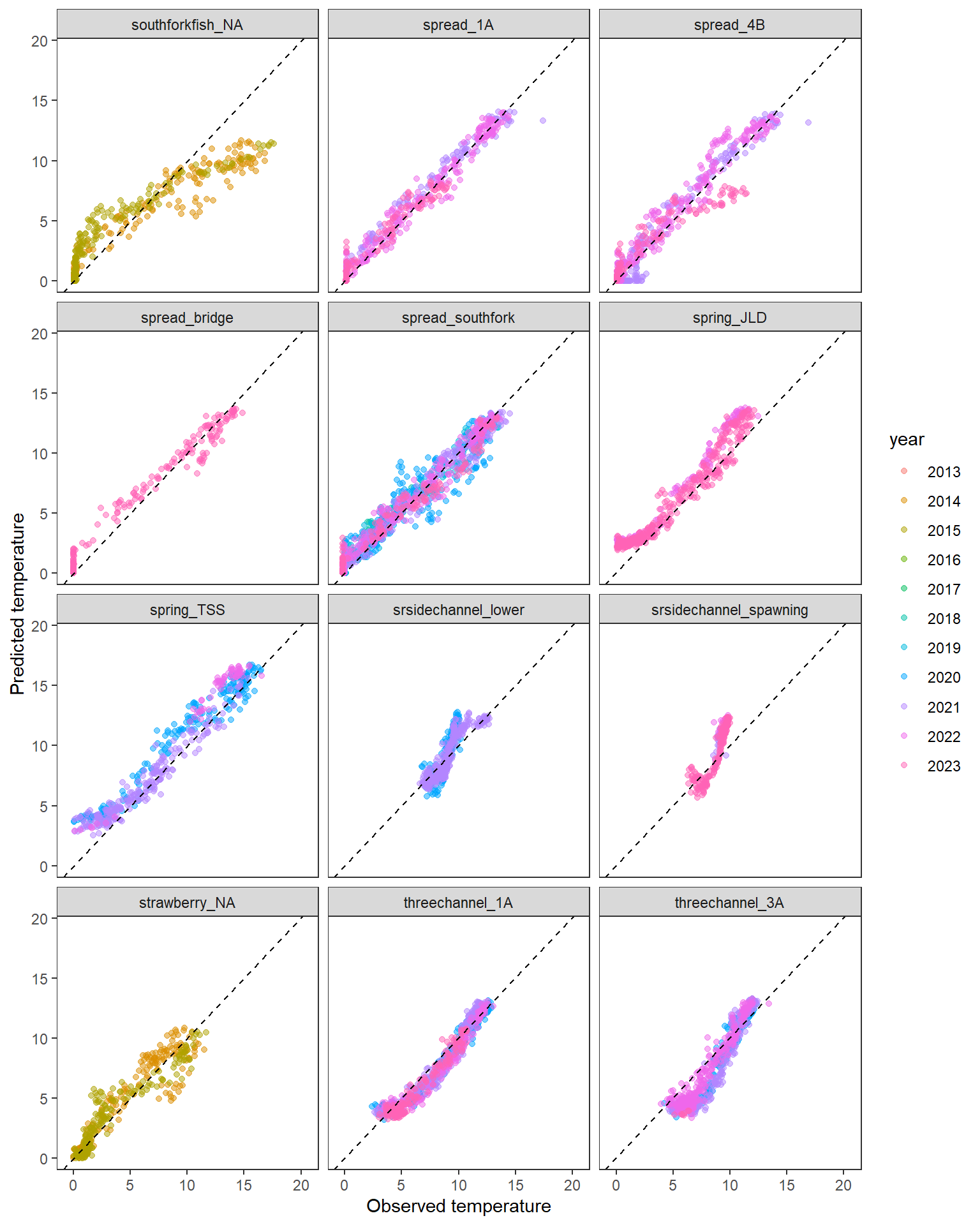
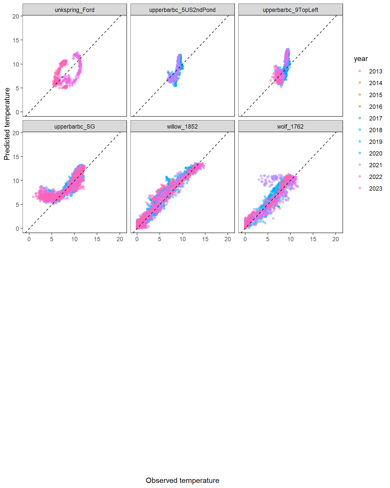
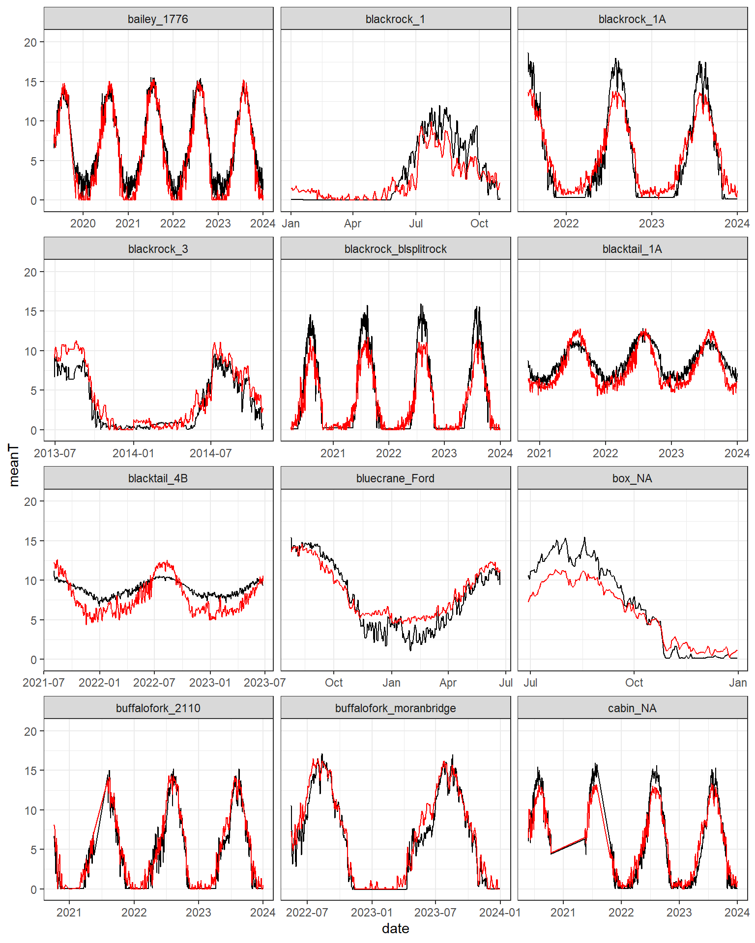
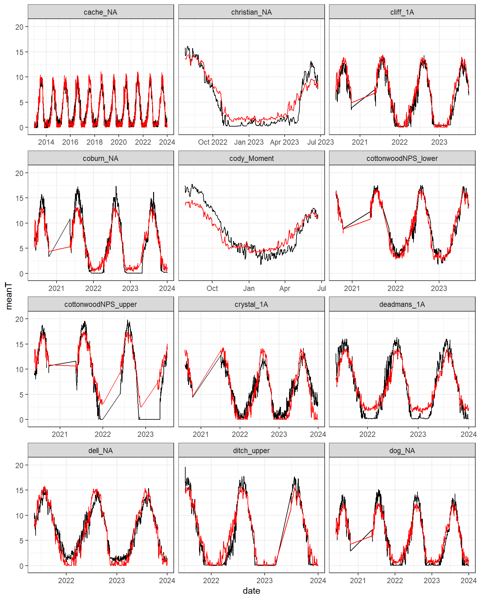
Annual pattern of residuals is generally consistent among years, within sites. Strong autocorrelation

3.4 Model residuals

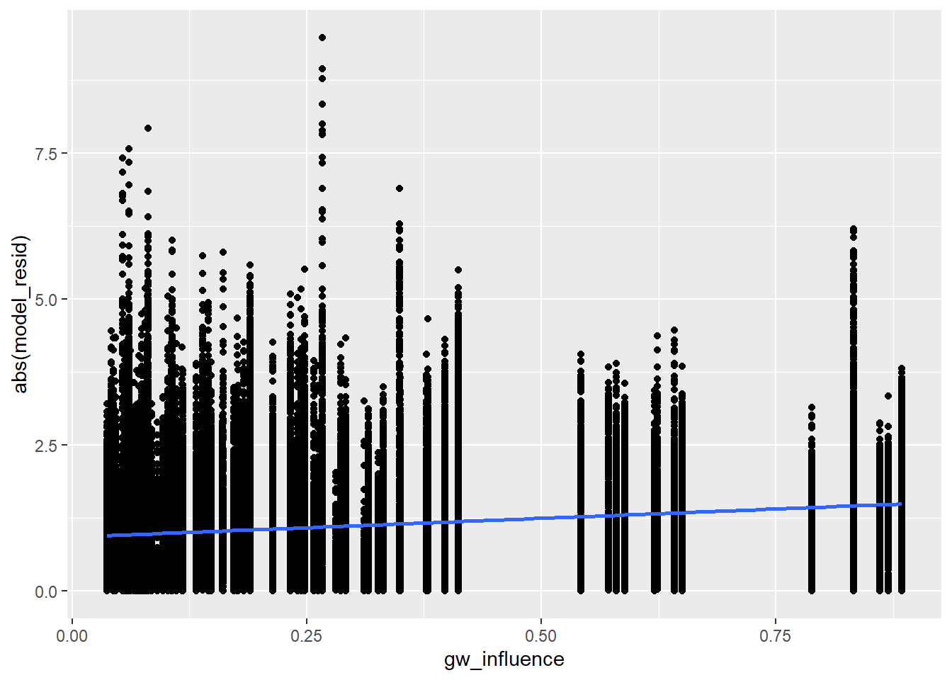
Absolute residuals by groundwater input

Code

summary(lm(abs(model_resid) ~ abs(model_resid_lag) + gw_influence, data = dat))


Call:
lm(formula = abs(model_resid) ~ abs(model_resid_lag) + gw_influence, 
    data = dat)

Residuals:
    Min      1Q  Median      3Q     Max 
-3.2751 -0.2558 -0.0380  0.2549  4.5355 

Coefficients:
                     Estimate Std. Error t value Pr(>|t|)    
(Intercept)          0.148783   0.003373   44.11   <2e-16 ***
abs(model_resid_lag) 0.838719   0.002045  410.17   <2e-16 ***
gw_influence         0.106627   0.008510   12.53   <2e-16 ***
---
Signif. codes:  0 '***' 0.001 '**' 0.01 '*' 0.05 '.' 0.1 ' ' 1

Residual standard error: 0.4909 on 70337 degrees of freedom
  (284 observations deleted due to missingness)
Multiple R-squared:  0.7122,    Adjusted R-squared:  0.7122 
F-statistic: 8.703e+04 on 2 and 70337 DF,  p-value: < 2.2e-16

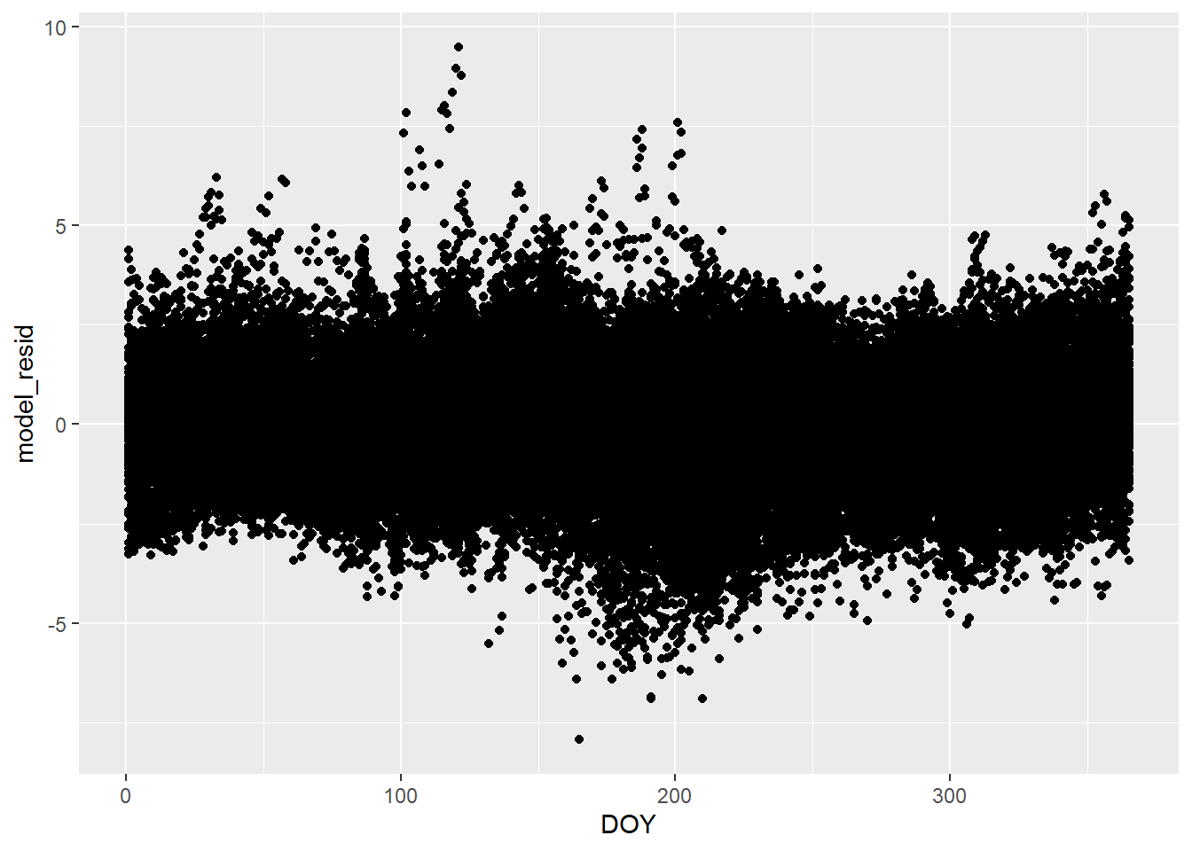
Code

dat %>%
  ggplot(aes(x = gw_influence, y = abs(model_resid))) +
  geom_point() +
  theme(legend.position = "none") +
  geom_smooth(method = "lm")

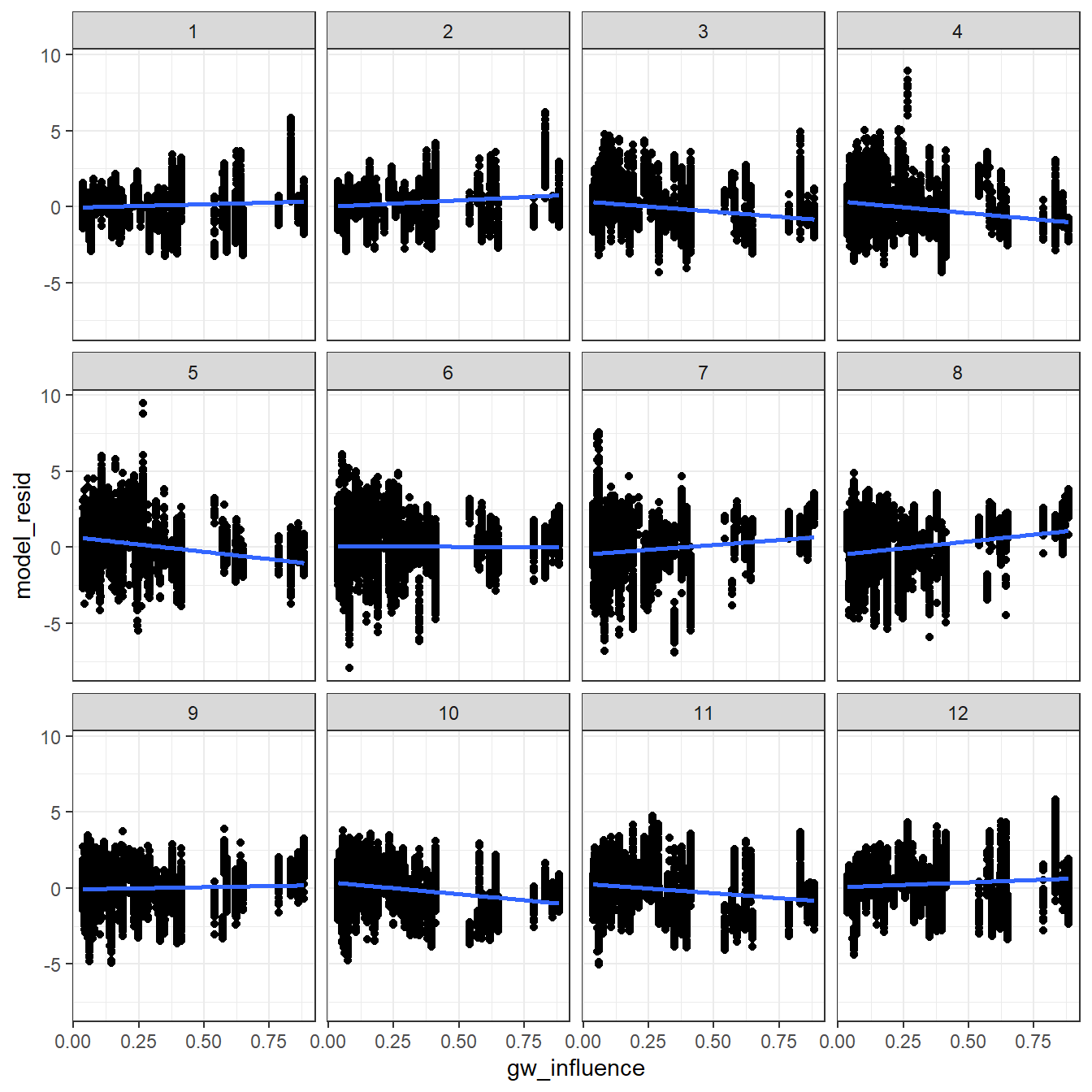
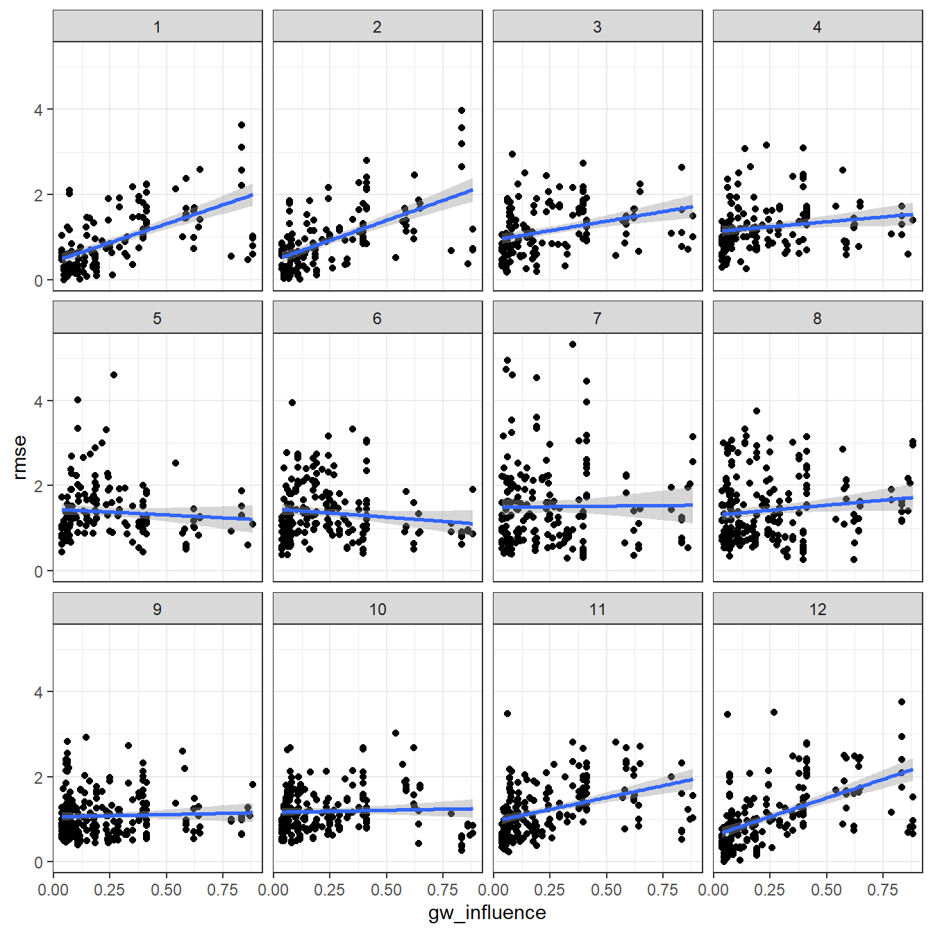
Residuals by groundwater and month

Code

dat %>%
  ggplot(aes(x = gw_influence, y = model_resid)) + 
  geom_point() +
  geom_smooth(method = "lm") +
  facet_wrap(~tim.month) + 
  theme_bw()

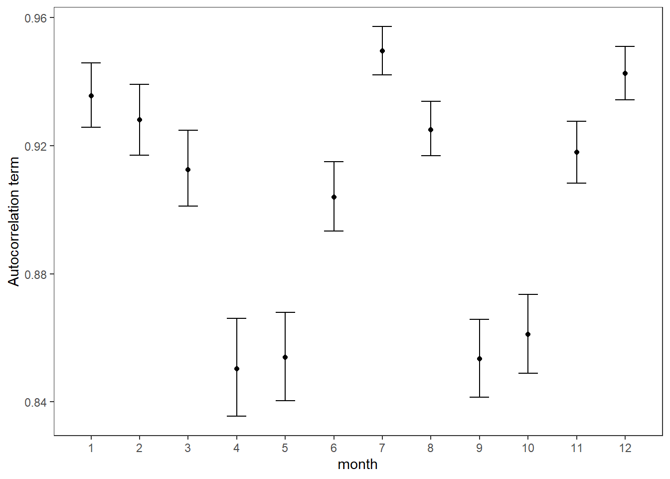
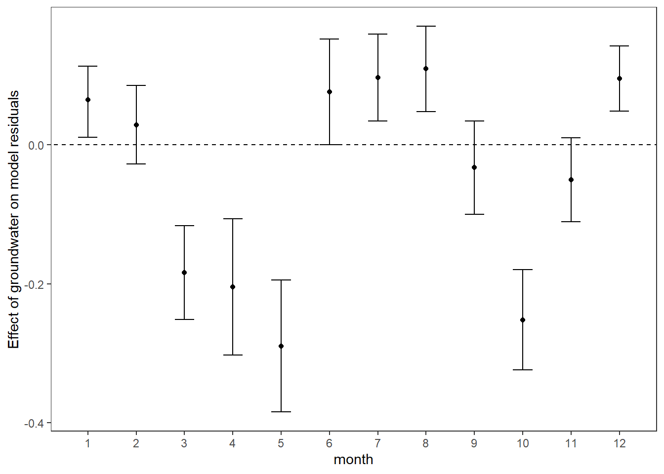
Explore time varying effects of groundwater on model residuals (linear mixed effects model includes lagged/autocorrelation term and random intercepts for year).

Code

# fit mixed effects models in a loop, independently for each month: residuals as a function of lagged residuals, site-level groundwater influence, and random intercepts for year
modlist <- list()
for (i in 1:12) {
  modlist[[i]] <- lmer(model_resid ~ model_resid_lag + gw_influence + (1|year), data = dat %>% filter(tim.month == i))
}

# empty tibble to store coefficients
efftib <- tibble(month = 1:12, 
                 mean.gw = rep(NA, 12),
                 lower.gw = rep(NA, 12),
                 upper.gw = rep(NA, 12), 
                 
                 mean.ac = rep(NA, 12),
                 lower.ac = rep(NA, 12),
                 upper.ac = rep(NA, 12))

# get coefficients, means and 95% confidence intervals
for (i in 1:12) {
  efftib$mean.gw[i] <- fixef(modlist[[i]])[3]
  efftib$lower.gw[i] <- confint(modlist[[i]])[5,1]
  efftib$upper.gw[i] <- confint(modlist[[i]])[5,2]
  
  efftib$mean.ac[i] <- fixef(modlist[[i]])[2]
  efftib$lower.ac[i] <- confint(modlist[[i]])[4,1]
  efftib$upper.ac[i] <- confint(modlist[[i]])[4,2]
}

# plot autocorrelation terms
efftib %>%
  ggplot() +
  geom_point(aes(x = month, y = mean.ac)) +
  geom_errorbar(aes(x = month, ymin = lower.ac, ymax = upper.ac), width = 0.4) +
  geom_abline(intercept = 0, slope = 0, linetype = "dashed") +
  theme_bw() + theme(panel.grid = element_blank()) + 
  ylab("Autocorrelation term") +
  scale_x_continuous(breaks = c(1:12))

Code

# plot groundwater effects
efftib %>%
  ggplot() +
  geom_point(aes(x = month, y = mean.gw)) +
  geom_errorbar(aes(x = month, ymin = lower.gw, ymax = upper.gw), width = 0.4) +
  geom_abline(intercept = 0, slope = 0, linetype = "dashed") +
  theme_bw() + theme(panel.grid = element_blank()) + 
  ylab("Effect of groundwater on model residuals") +
  scale_x_continuous(breaks = c(1:12))

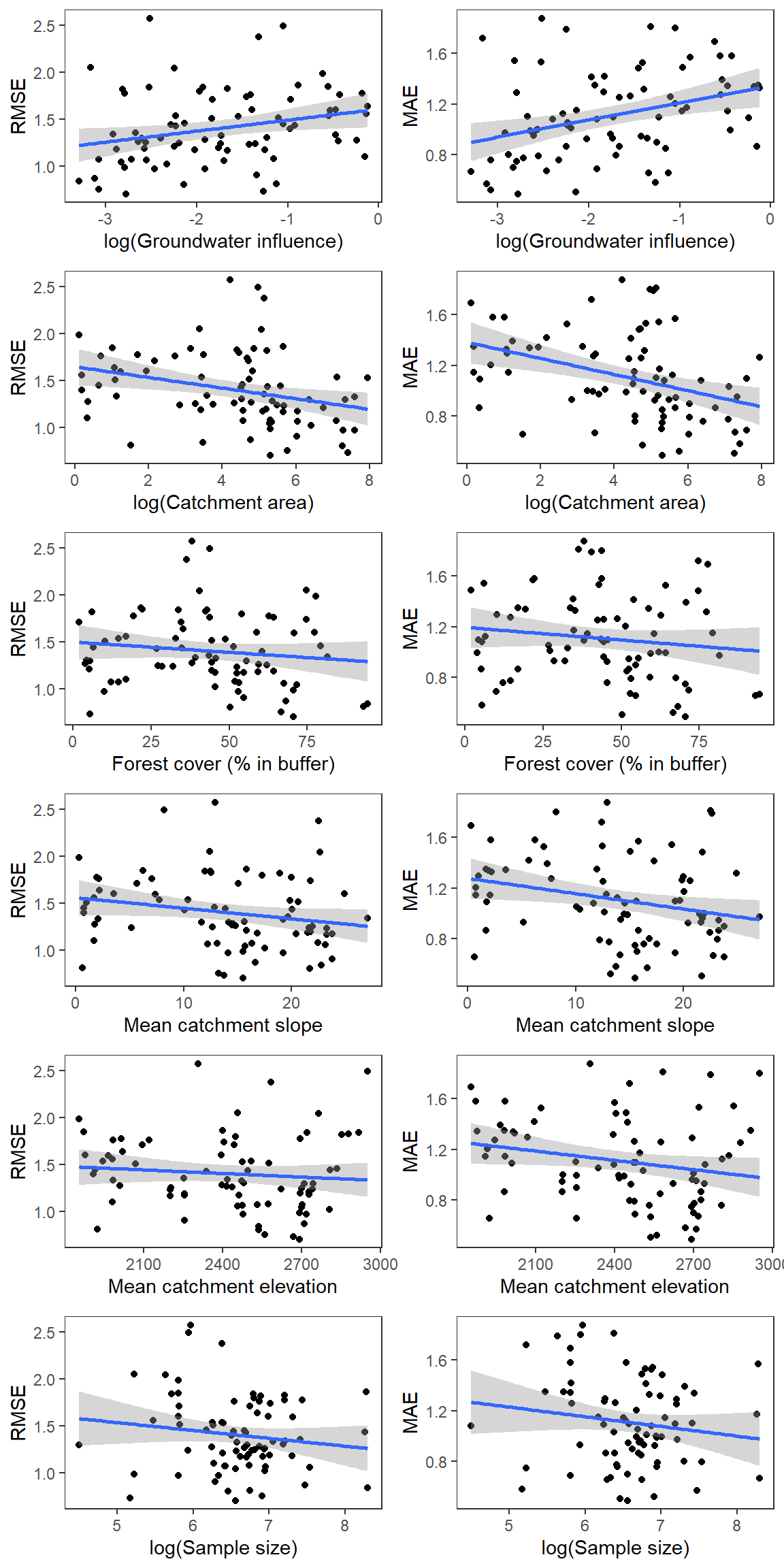
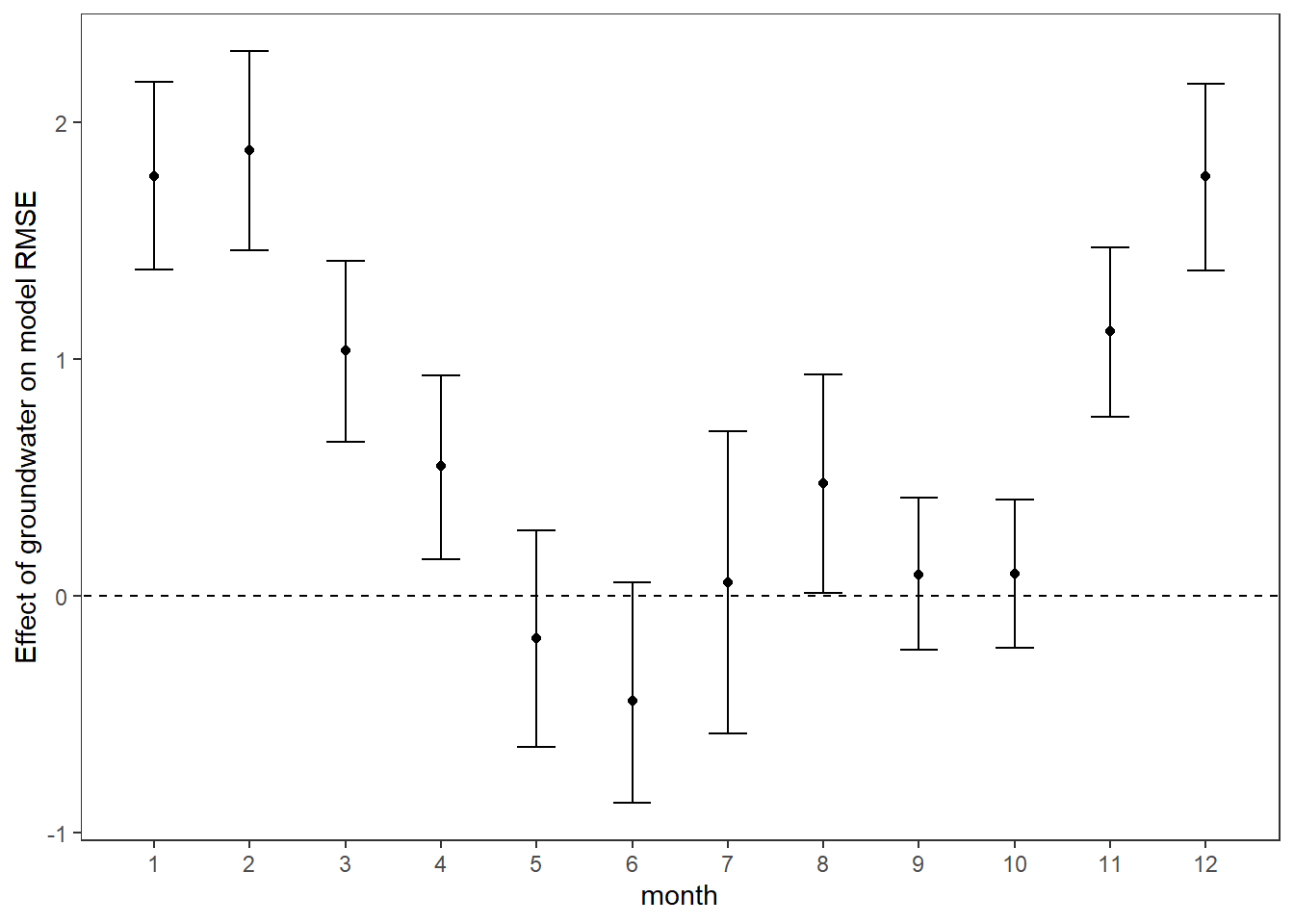
3.5 Model RMSE

Alternatively, we can model monthly RMSE, rather than the raw residuals. This eliminates the need for an autocorrelation term and is based on a coarser measure of predictive accuracy (is using/modeling all residuals pseudoreplication), but limits our ability to discriminate between under vs over-estimates/predictions.

3.5.1 Monthly models

Summarize data by site, year, and month

Code

errorterms <- dat %>%
  group_by(site, year, tim.month) %>%
  summarize(gw_influence = mean(gw_influence),
            h2oAreaKm2_log = mean(h2oAreaKm2_log),
            forest_buff_perc = mean(forest_buff_perc),
            h2o_slope_mean = mean(h2o_slope_mean),
            h2o_elev_mean = mean(h2o_elev_mean),
            sampsize = n(),
            rmse = sqrt(mean((model_resid)^2)),
            mae = mean(abs(model_resid))) %>%
  ungroup() %>%
  filter(sampsize >= 28)

RMSE by groundwater and month

Code

errorterms %>%
  ggplot(aes(x = gw_influence, y = rmse)) + 
  geom_point() +
  geom_smooth(method = "lm") +
  facet_wrap(~tim.month) + 
  theme_bw()

Fit linear mixed effects models in a loop, independently for each month: RMSE as a function of site-level groundwater influence and random intercepts for year

Code

modlist <- list()
for (i in 1:12) {
  modlist[[i]] <- lmer(rmse ~ gw_influence + (1|year), data = errorterms %>% filter(tim.month == i))
}

# empty tibble to store coefficients
efftib <- tibble(month = 1:12, 
                 mean.gw = rep(NA, 12),
                 lower.gw = rep(NA, 12),
                 upper.gw = rep(NA, 12))

# get coefficients, means and 95% confidence intervals
for (i in 1:12) {
  efftib$mean.gw[i] <- fixef(modlist[[i]])[2]
  efftib$lower.gw[i] <- confint(modlist[[i]])[4,1]
  efftib$upper.gw[i] <- confint(modlist[[i]])[4,2]
}

# plot groundwater effects
efftib %>%
  ggplot() +
  geom_point(aes(x = month, y = mean.gw)) +
  geom_errorbar(aes(x = month, ymin = lower.gw, ymax = upper.gw), width = 0.4) +
  geom_abline(intercept = 0, slope = 0, linetype = "dashed") +
  theme_bw() + theme(panel.grid = element_blank()) + 
  ylab("Effect of groundwater on model RMSE") +
  scale_x_continuous(breaks = c(1:12))

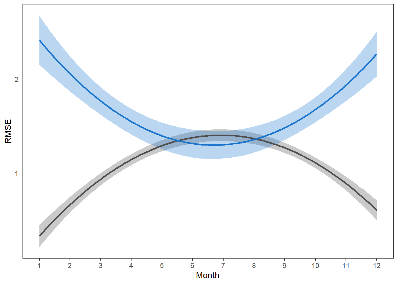
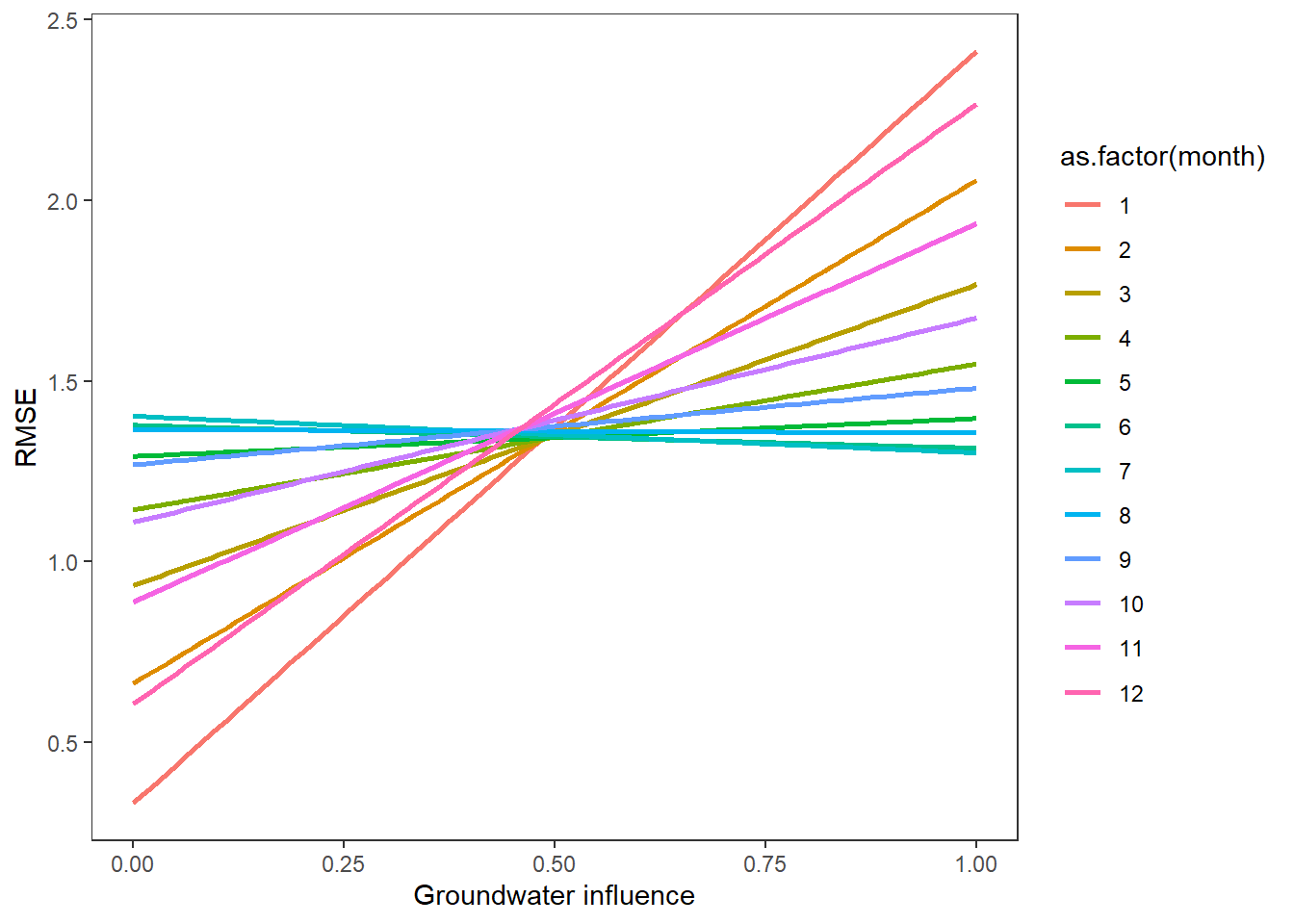
3.5.2 Interaction model

Same, but different: model the interaction between month and groundwater directly:

Code

# errorterms %>% 
#   group_by(tim.month) %>%
#   summarize(rmse = mean(rmse)) %>%
#   ggplot(aes(x = tim.month, y = rmse)) +
#   geom_point() +
#   geom_line() +
#   theme_bw() + theme(panel.grid = element_blank()) +
#   xlab("Month") + ylab("Mean RMSE") +
#   scale_x_continuous(breaks = c(1:12))

errorterms %>% 
  #filter(gw_influence < 0.15) %>%
  ggplot(aes(x = tim.month, y = rmse, color = gw_influence)) + 
  geom_point() +
  geom_line(aes(group = interaction(site, year), color = gw_influence)) +
  theme_bw() + theme(panel.grid = element_blank()) +
  xlab("Month") + ylab("RMSE") +
  scale_x_continuous(breaks = c(1:12))

Based on the plot of the data above, fit a linear interaction model with second order polynomial for groundwater influence:

Code

mymod <- lm(rmse ~ gw_influence + tim.month + I(tim.month^2) + gw_influence*tim.month + gw_influence*I(tim.month^2), data = errorterms)
summary(mymod)


Call:
lm(formula = rmse ~ gw_influence + tim.month + I(tim.month^2) + 
    gw_influence * tim.month + gw_influence * I(tim.month^2), 
    data = errorterms)

Residuals:
    Min      1Q  Median      3Q     Max 
-1.6619 -0.4619 -0.1222  0.3325  3.9495 

Coefficients:
                             Estimate Std. Error t value Pr(>|t|)    
(Intercept)                 -0.062195   0.081936  -0.759    0.448    
gw_influence                 2.900940   0.236269  12.278   <2e-16 ***
tim.month                    0.424496   0.027813  15.263   <2e-16 ***
I(tim.month^2)              -0.030731   0.002054 -14.965   <2e-16 ***
gw_influence:tim.month      -0.884712   0.081323 -10.879   <2e-16 ***
gw_influence:I(tim.month^2)  0.065111   0.006025  10.807   <2e-16 ***
---
Signif. codes:  0 '***' 0.001 '**' 0.01 '*' 0.05 '.' 0.1 ' ' 1

Residual standard error: 0.6583 on 2167 degrees of freedom
Multiple R-squared:  0.1348,    Adjusted R-squared:  0.1328 
F-statistic: 67.54 on 5 and 2167 DF,  p-value: < 2.2e-16

Plot the model predictions:

Code

mymonths <- seq(from = 1, to = 12, length.out = 100)
preds_gw0 <- predict(mymod, newdata = list(gw_influence = rep(0, times = 100), tim.month = mymonths),
                     interval = "confidence", level = 0.95)
preds_gw1 <- predict(mymod, newdata = list(gw_influence = rep(1, times = 100), tim.month = mymonths),
                     interval = "confidence", level = 0.95)

ggplot() + 
  geom_ribbon(aes(x = mymonths, ymin = preds_gw0[,2], ymax = preds_gw0[,3]), 
              color = NA, fill = "grey30", alpha = 0.3) +
  geom_ribbon(aes(x = mymonths, ymin = preds_gw1[,2], ymax = preds_gw1[,3]), 
              linewidth = 1, color = NA, fill = "dodgerblue3", alpha = 0.3) +
  geom_line(aes(x = mymonths, y = preds_gw0[,1]), linewidth = 1, color = "grey30") +
  geom_line(aes(x = mymonths, y = preds_gw1[,1]), linewidth = 1, color = "dodgerblue3") +
  theme_bw() + theme(panel.grid = element_blank()) +
  xlab("Month") + ylab("RMSE") +
  scale_x_continuous(breaks = c(1:12))

Derive the month-specific effect of groundwater on RMSE

Code

mygw <- seq(from = 0, to = 1, length.out = 100)
predlist <- list()
for (i in 1:12) {
  preds <- predict(mymod, newdata = list(gw_influence = mygw, tim.month = rep(i, times = 100)),
                   interval = "confidence", level = 0.95)
  predlist[[i]] <- tibble(month = rep(i, times = 100),
                          gw = mygw,
                          fit = preds[,1],
                          lwr = preds[,2],
                          upr = preds[,3])
}
predtib <- bind_rows(predlist)

predtib %>%
  ggplot(aes(x = gw, y = fit, group = as.factor(month), color = as.factor(month))) +
  geom_line(linewidth = 1) +
  theme_bw() + theme(panel.grid = element_blank()) +
  xlab("Groundwater influence") + ylab("RMSE")

Note that these results generally match those above (results from the monthly RMSE models), but packages everything into a single model statement.