5  Simple Growth Regime

Purpose: Derive and visualize the growth regime in two alternative habitat patches sensu Armstrong et al. (2021).

Source dependencies

Load pre-calculated growth

load("data/wt.growth.array.RData")

5.1 Simple growth regime

Derive a generic growth regime for a 10 gram fish, sensu Armstrong et al. (2021). For simplicity, I did not simulate changing growth potential due to increase in fish mass over the course of the year, as in the NCC paper.

Notes:

• In these ~simple scenarios, growth potential for the “optimal mover” is just calculated from the maximum of that across the two habitats. No need to simulate habitat selection/movement.

5.1.1 Get growth potential

Objects

waterTemps <- cbind("pid" = seq(1, length(seq(0.1, 25, 0.1))),"WT" = seq(0.1, 25, 0.1))
rations <- seq(0.001, 0.4, 0.001)
weights <- seq(0.25, 1500, 0.25)

length(rations)

[1] 400

which(weights == 10)

[1] 40

Get growth potential by temperature for a 10 gram fish, fed at ~max ration

# get relative growth rates for a 10 g fish across range of water temps
grate_df <- tibble(temp = waterTemps[,2],
                   grate_ggd = wt.growth[,400,40]) %>%
  mutate(temp = trimws(temp))

# calculate growth potential (g/d/d) and cumulative growth (g) across warm and cold patches and for an "optimal mover"
growthregime_df <- habitat_df %>%
  mutate(temp_warm = trimws(temp_warm),
         temp_cold = trimws(temp_cold)) %>%
  left_join(grate_df, by = c("temp_warm" = "temp")) %>% rename(grpot_warm = grate_ggd) %>%
  left_join(grate_df, by = c("temp_cold" = "temp")) %>% rename(grpot_cold = grate_ggd) %>%
  mutate(grpot_track = pmax(grpot_warm, grpot_cold)) %>%
  mutate(cumul_growth_warm = cumsum(grpot_warm*10),
         cumul_growth_cold = cumsum(grpot_cold*10),
         cumul_growth_track = cumsum(grpot_track*10),
         habitat = case_when(
           grpot_cold > grpot_warm ~ "cold",
           grpot_warm > grpot_cold ~ "warm",
           TRUE ~ "tie"
         ))
  
head(growthregime_df)

# A tibble: 6 × 15
  date         doy temp_warm temp_cold ration_warm ration_cold pcmax_warm
  <date>     <int> <chr>     <chr>           <dbl>       <dbl>      <dbl>
1 2024-01-01     1 0.5       0.3               0.1         0.1        0.5
2 2024-01-02     2 0.5       0.3               0.1         0.1        0.5
3 2024-01-03     3 0.5       0.3               0.1         0.1        0.5
4 2024-01-04     4 0.5       0.3               0.1         0.1        0.5
5 2024-01-05     5 0.5       0.3               0.1         0.1        0.5
6 2024-01-06     6 0.5       0.3               0.1         0.1        0.5
# ℹ 8 more variables: pcmax_cold <dbl>, grpot_warm <dbl>, grpot_cold <dbl>,
#   grpot_track <dbl>, cumul_growth_warm <dbl>, cumul_growth_cold <dbl>,
#   cumul_growth_track <dbl>, habitat <chr>

5.1.2 Visualize output

Plot growth regimes (growth potential and g/g/d)

p1 <- growthregime_df %>% ggplot() +
  geom_line(aes(x = date, y = grpot_warm), col = 2) +
  geom_line(aes(x = date, y = grpot_cold), col = 4) +
  theme_bw() +
  xlab("Date") +
  ylab("Growth potential (g/g/day)") +
  labs(title = "Warm vs. cold habitats")

p2 <- growthregime_df %>% ggplot() +
  geom_line(aes(x = date, y = grpot_track), col = 1, linetype = "dashed") +
  theme_bw() +
  xlab("Date") +
  ylab("Growth potential (g/g/day)") +
  labs(title = "Optimal mover")

ggarrange(p1, p2, ncol = 2)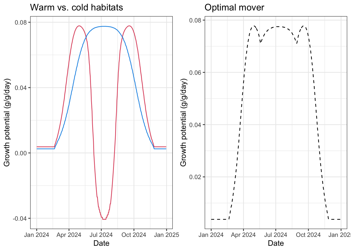

Plot cumulative growth

growthregime_df %>% ggplot() +
  geom_line(aes(x = date, y = cumul_growth_warm, color = "Warm resident")) +
  geom_line(aes(x = date, y = cumul_growth_cold, color = "Cold resident")) +
  geom_line(aes(x = date, y = cumul_growth_track, color = "Optimal mover"), linetype = "dashed") +
  scale_color_manual(values = c("Warm resident" = 2, "Cold resident" = 4, "Optimal mover" = 1)) +
  theme_bw() +
  xlab("Date") +
  ylab("Cumulative growth (g)")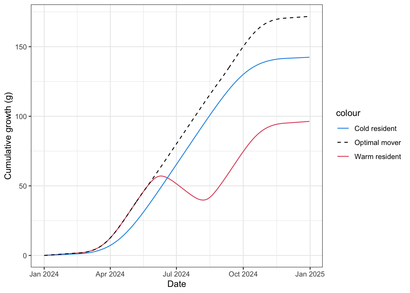

Plot habitat use, i.e., temporal change in the habitat where growth potential is maximized.

growthregime_df %>% 
  mutate(habitat_num = as.numeric(as.factor(habitat))) %>%
  ggplot() +
  geom_line(aes(x = date, y = habitat_num)) +
  geom_point(aes(x = date, y = habitat_num, color = habitat)) +
  theme_bw() +
  scale_color_manual(values = c("cold" = 4, "warm" = 2)) +
  xlab("Date") +
  ylab("Habitat with max. GP (cold = 1, warm = 2)")

Contributions of warm vs. cold patches

# time
growthregime_df %>% 
  group_by(habitat) %>%
  summarize(ndays = n()) %>%
  mutate(habitat = factor(habitat)) %>%
  ggplot() +
  geom_bar(aes(x = habitat, y = ndays/dim(growthregime_df)[1], fill = habitat), stat = "identity") +
  theme_bw() + theme(legend.position = "none") +
  scale_fill_manual(values = c("cold" = 4, "warm" = 2)) +
  ylab("Proportion of time spent in cold vs. warm habitats")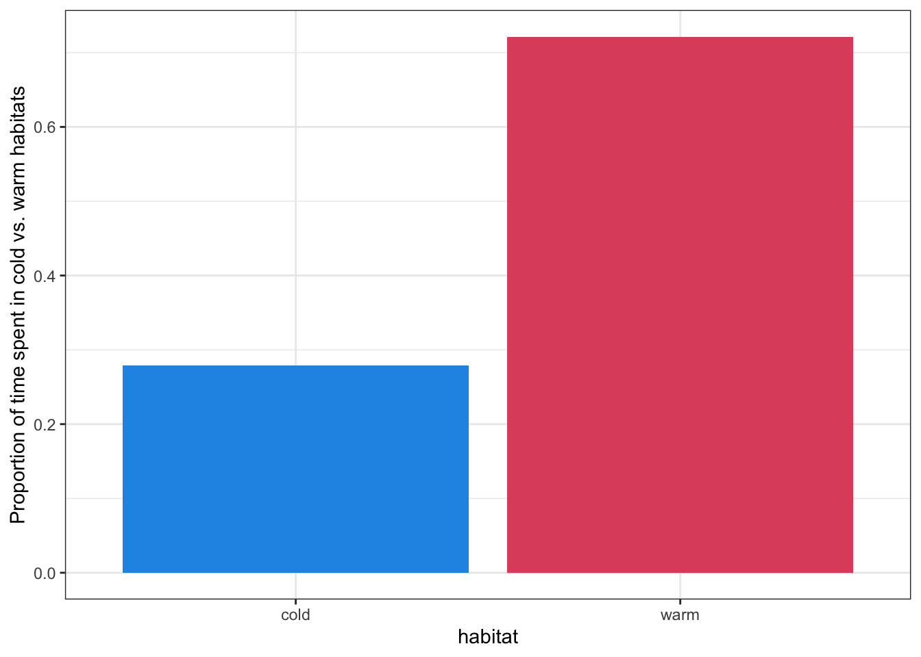

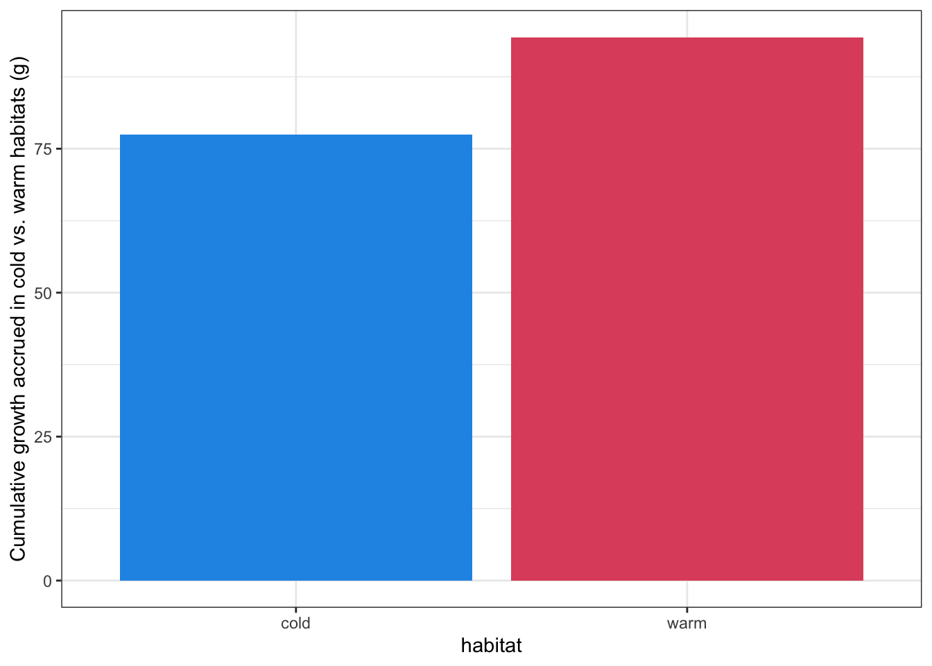
# cumulative growth accrued
growthregime_df %>% 
  group_by(habitat) %>%
  summarize(cumul_grpot = sum(grpot_track*10)) %>%
  mutate(habitat = factor(habitat)) %>%
  ggplot() +
  geom_bar(aes(x = habitat, y = cumul_grpot, fill = habitat), stat = "identity") +
  theme_bw() + theme(legend.position = "none") +
  scale_fill_manual(values = c("cold" = 4, "warm" = 2)) +
  ylab("Cumulative growth accrued in cold vs. warm habitats (g)")