2  Simulate Habitat

if any changes are made, need to re-run qmd_to_r_script() function at end, in console

Purpose: This script simulates habitat conditions (temperature and food availability) for a simple, spatially-implicit habitat network consisting of two patches.

Notes:

• In theory, habitat network is generalizable and can be expanded to include as many patches as needed. But in doing so we will need to update the simulation to allow more than 2 patches.
• We can specify food available in one of two ways, ration size in g/g/d or proportion of maximum consumption (P_C_max). Fullerton’s IBM in Armstrong et al. (2021) sets a constant ration size (g/g/d) in each patch, and varies this from upstream to downstream. The problem with this is that is that it forces small fish to feed way below C_max, but as fish grow and allometric C_max declines, fish feed much closer to or at C_max. Therefore, growth rates are low and constraining for small fish, but increase as fish grow larger, such that fish are less constrained by food availability.
  • Many researchers using bioenergetics models simply set a constant P_C_max, then estimate growth from that. But the problem with this, as Railsback points out, is that under warmer conditions fish are able to attain higher ration sizes simply because of the temperature dependence function: C = Cmax * p * f(T). Thus, there is no way to separate ration size from habitat temperature using a constant P_C_max.
  • Instead, we can simply modify the temperature dependence function to set some threshold P_C_max. Basically, temperature acts on ration/consumption up to some threshold value of P_C_max, above which body size alone limits consumption (via allometric C_max).

2.1 Configuration

nyears_burnin <- 20
nyears_experiment <- 20

mindate <- as.Date("2001-05-01")
maxdate <- mindate + years(nyears_burnin) + years(nyears_experiment)

dates <- seq(mindate, maxdate, by="day")
n <- length(dates)
doy <- as.numeric(format(dates, "%j")) # Day of year

Current configuration:

• Temp: simple warm and cold patches…cold regime is simply 60% of daily warm regime values. No noise.
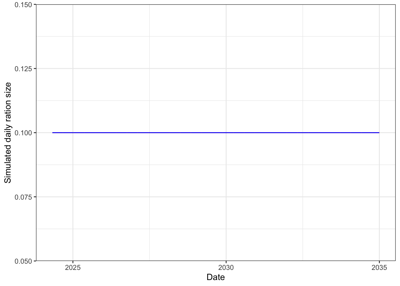
• P_Cmax: constant proportion of maximum consumption, same in each patch. No noise.

2.2 Temperature

Simulate thermal regimes as annual sine waves. Cold vs. Warm using simple multiplier.

# Set seed for reproducibility
set.seed(123)

# 2. Simulate Stream Temperature (Sine wave + Noise)
# Parameters: Midpoint, Amplitude, Offset
base_temp <- 11        # Average annual temperature
amplitude <- 14         # Seasonal fluctuation amplitude
# Peak temperature occurs late in the year (July/Aug)
stream_temp <- base_temp + amplitude * sin(2 * pi * (doy - 100) / 365)

# 3. Add random noise (daily weather variation)
noise <- rnorm(n, mean = 0, sd = 0) # no variation for simplicity
simulated_temp <- stream_temp + noise

# 4. Force values near 0 to small postive, max = 25
simulated_temp[simulated_temp < 0.5] <- 0.5
simulated_temp[simulated_temp > 25] <- 25

# 4. Simulate cold regime using a multiplier
simulated_temp_cold <- simulated_temp*0.6

# 4. Create Data Frame
habitat_df <- tibble(date = dates, 
                     doy = doy, 
                     dayofsim = 1:length(dates),
                     temp_warm = round(simulated_temp, digits = 1), 
                     temp_cold = round(simulated_temp_cold, digits = 1))

# 5. Plot the simulation
summer_shading <- data.frame(
  xmin = as.Date(paste0(unique(format(habitat_df$date, "%Y")), "-06-01")),
  xmax = as.Date(paste0(unique(format(habitat_df$date, "%Y")), "-08-31")),
  ymin = -Inf, ymax = Inf
)

habitat_df %>% ggplot() +
  geom_rect(data = summer_shading,
            aes(xmin = xmin, xmax = xmax, ymin = ymin, ymax = ymax),
            fill = "grey", alpha = 0.3, inherit.aes = FALSE) +
  geom_line(aes(x = date, y = temp_warm), color = "red") +
  geom_line(aes(x = date, y = temp_cold), color = "blue") +
  theme_bw() + 
  xlab("Date") + 
  ylab("Simulated daily stream temperature (deg C)") + 
  labs(title = "Daily stream temperature with Jun-Aug shaded")

# function to retrieve water temperature in patch = patch and at doy/time = t
get_patchtemp <- function(t, patch) {
  if (patch == "warm") {
    habitat_df$temp_warm[habitat_df$dayofsim == t]
  } else {
    habitat_df$temp_cold[habitat_df$dayofsim == t]
  }
}

2.3 Patch Parameters

Patch-specific parameters that govern maximum consumption, density dependence, patch area, and maximum survival probability. These are stored as time series columns in habitat_df so they can vary across years (e.g., after a burn-in period) to simulate habitat change experiments.

# --- Maximum proportion of maximum consumption ---
pcmax_warm_val <- 0.5
pcmax_cold_val <- 0.5

# --- Patch area (arbitrary units; keep at 1.0 to preserve default behaviour) ---
A_warm_val <- 1.0
A_cold_val <- 1.0

# --- Half-saturation density for hyperbolic ration reduction ---
# Competitor density (fish per unit area) at which ration is halved
K_warm_val <- 500
K_cold_val <- 500

# --- Maximum daily survival probability (size-based survival ceiling) ---
S_max_warm_val <- 0.9994
S_max_cold_val <- 0.9994

# Append as time-invariant columns (replace with time-varying vectors to simulate change)
habitat_df <- habitat_df %>%
  mutate(
    pcmax_warm = pcmax_warm_val,
    pcmax_cold = pcmax_cold_val,
    A_warm     = A_warm_val,
    A_cold     = A_cold_val,
    K_warm     = K_warm_val,
    K_cold     = K_cold_val,
    S_max_warm = S_max_warm_val,
    S_max_cold = S_max_cold_val
  )

2.4 Set-up Habitat Change Experiment

After the burn-in period, one or more patch parameters can be ramped to new target values. Set a target to NA to leave that parameter unchanged. ramp_years = 0 gives an immediate step change; any positive value linearly interpolates from the end-of-burn-in value to the target over that many years, then holds the target for the remainder of the experiment.

# First row of the experiment period
exp_start_date <- mindate + lubridate::years(nyears_burnin)
d_exp_start    <- which(habitat_df$date == exp_start_date)

# --- Target values for each parameter (NA = no change) ---
pcmax_warm_target  <- NA
pcmax_cold_target  <- NA
A_warm_target      <- 2
A_cold_target      <- 0
K_warm_target      <- NA
K_cold_target      <- NA
S_max_warm_target  <- NA
S_max_cold_target  <- NA

# --- Transition: 0 = step change; > 0 = linear ramp over this many years ---
ramp_years <- nyears_experiment

# Linearly ramps col from its end-of-burn-in value to target_val over ramp_yrs years,
# then holds target_val for the remainder of the experiment period.
apply_ramp <- function(col, d_start, target_val, ramp_yrs) {
  baseline  <- col[d_start - 1]
  n_ramp    <- max(round(ramp_yrs * 365.25), 1)  # min 1 to avoid /0
  exp_idx   <- d_start:length(col)
  ramp_frac <- pmin(seq_along(exp_idx) / n_ramp, 1)
  col[exp_idx] <- baseline + (target_val - baseline) * ramp_frac
  col
}

params_to_change <- list(
  pcmax_warm = pcmax_warm_target,
  pcmax_cold = pcmax_cold_target,
  A_warm     = A_warm_target,
  A_cold     = A_cold_target,
  K_warm     = K_warm_target,
  K_cold     = K_cold_target,
  S_max_warm = S_max_warm_target,
  S_max_cold = S_max_cold_target
)

for (param in names(params_to_change)) {
  target <- params_to_change[[param]]
  if (!is.na(target)) {
    habitat_df[[param]] <- apply_ramp(habitat_df[[param]], d_exp_start, target, ramp_years)
  }
}

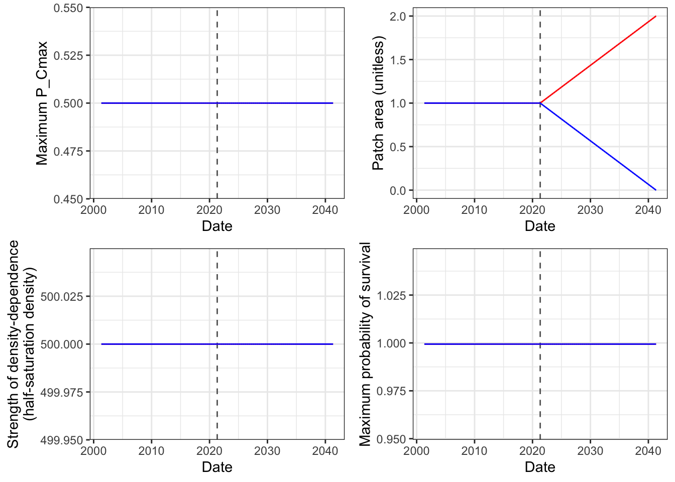
Plot time series of habitat conditions

p1 <- habitat_df %>% ggplot() +
  geom_vline(xintercept = exp_start_date, linetype = "dashed", color = "grey40") +
  geom_line(aes(x = date, y = pcmax_warm), color = "red") +
  geom_line(aes(x = date, y = pcmax_cold), color = "blue") +
  theme_bw() +
  xlab("Date") +
  ylab("Maximum P_Cmax")

p2 <- habitat_df %>% ggplot() +
  geom_vline(xintercept = exp_start_date, linetype = "dashed", color = "grey40") +
  geom_line(aes(x = date, y = A_warm), color = "red") +
  geom_line(aes(x = date, y = A_cold), color = "blue") +
  theme_bw() +
  xlab("Date") +
  ylab("Patch area (unitless)")

p3 <- habitat_df %>% ggplot() +
  geom_vline(xintercept = exp_start_date, linetype = "dashed", color = "grey40") +
  geom_line(aes(x = date, y = K_warm), color = "red") +
  geom_line(aes(x = date, y = K_cold), color = "blue") +
  theme_bw() +
  xlab("Date") +
  ylab("Strength of density-dependence\n(half-saturation density)")

p4 <- habitat_df %>% ggplot() +
  geom_vline(xintercept = exp_start_date, linetype = "dashed", color = "grey40") +
  geom_line(aes(x = date, y = S_max_warm), color = "red") +
  geom_line(aes(x = date, y = S_max_cold), color = "blue") +
  theme_bw() +
  xlab("Date") +
  ylab("Maximum probability of survival")

egg::ggarrange(p1, p2, p3, p4, nrow = 2, ncol = 2)

2.5 View data

str(habitat_df)

tibble [14,611 × 13] (S3: tbl_df/tbl/data.frame)
 $ date      : Date[1:14611], format: "2001-05-01" "2001-05-02" ...
 $ doy       : num [1:14611] 121 122 123 124 125 126 127 128 129 130 ...
 $ dayofsim  : int [1:14611] 1 2 3 4 5 6 7 8 9 10 ...
 $ temp_warm : num [1:14611] 16 16.2 16.4 16.6 16.8 17.1 17.3 17.5 17.7 17.9 ...
 $ temp_cold : num [1:14611] 9.6 9.7 9.8 10 10.1 10.2 10.4 10.5 10.6 10.7 ...
 $ pcmax_warm: num [1:14611] 0.5 0.5 0.5 0.5 0.5 0.5 0.5 0.5 0.5 0.5 ...
 $ pcmax_cold: num [1:14611] 0.5 0.5 0.5 0.5 0.5 0.5 0.5 0.5 0.5 0.5 ...
 $ A_warm    : num [1:14611] 1 1 1 1 1 1 1 1 1 1 ...
 $ A_cold    : num [1:14611] 1 1 1 1 1 1 1 1 1 1 ...
 $ K_warm    : num [1:14611] 500 500 500 500 500 500 500 500 500 500 ...
 $ K_cold    : num [1:14611] 500 500 500 500 500 500 500 500 500 500 ...
 $ S_max_warm: num [1:14611] 0.999 0.999 0.999 0.999 0.999 ...
 $ S_max_cold: num [1:14611] 0.999 0.999 0.999 0.999 0.999 ...

head(habitat_df)

# A tibble: 6 × 13
  date         doy dayofsim temp_warm temp_cold pcmax_warm pcmax_cold A_warm
  <date>     <dbl>    <int>     <dbl>     <dbl>      <dbl>      <dbl>  <dbl>
1 2001-05-01   121        1      16         9.6        0.5        0.5      1
2 2001-05-02   122        2      16.2       9.7        0.5        0.5      1
3 2001-05-03   123        3      16.4       9.8        0.5        0.5      1
4 2001-05-04   124        4      16.6      10          0.5        0.5      1
5 2001-05-05   125        5      16.8      10.1        0.5        0.5      1
6 2001-05-06   126        6      17.1      10.2        0.5        0.5      1
# ℹ 5 more variables: A_cold <dbl>, K_warm <dbl>, K_cold <dbl>,
#   S_max_warm <dbl>, S_max_cold <dbl>

2.6 Write R file

For sourcing later

#quarto::qmd_to_r_script("Habitat.qmd")