Code
ggplot(tempDataSyncS,aes(dOY,airTemp))+
geom_line(aes(color=factor(year))) +
facet_grid(year~riverOrdered)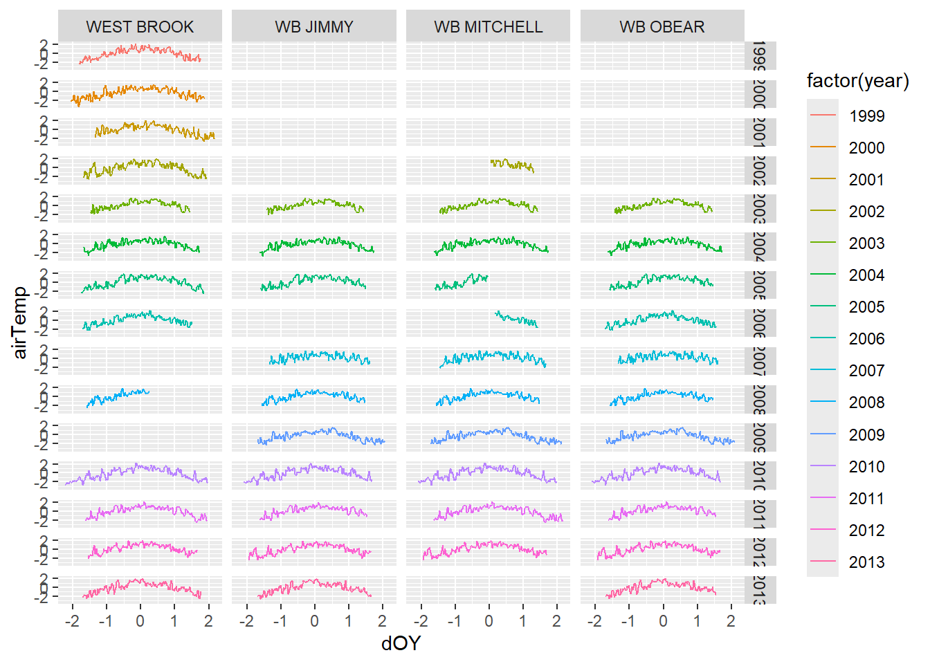
Purpose: fit stream temp model as in Letcher et al. (2016); modify JAGS model to estimate parameters hierarchically and check to make sure output matches.
Load fully formatted data used in Letcher et al. (2016) PeerJ ::: {.cell}
load("data/tempDataSyncSUsed.RData")
head(tempDataSyncS)
agency date AgencyID year fyear site fsite
1 MAUSGS 2003-04-15 WB JIMMY 2003 2003 MAUSGS_WB_JIMMY MAUSGS_WB_JIMMY
2 MAUSGS 2003-04-17 WB JIMMY 2003 2003 MAUSGS_WB_JIMMY MAUSGS_WB_JIMMY
3 MAUSGS 2003-04-18 WB JIMMY 2003 2003 MAUSGS_WB_JIMMY MAUSGS_WB_JIMMY
4 MAUSGS 2003-04-19 WB JIMMY 2003 2003 MAUSGS_WB_JIMMY MAUSGS_WB_JIMMY
5 MAUSGS 2003-04-20 WB JIMMY 2003 2003 MAUSGS_WB_JIMMY MAUSGS_WB_JIMMY
6 MAUSGS 2003-04-21 WB JIMMY 2003 2003 MAUSGS_WB_JIMMY MAUSGS_WB_JIMMY
date.1 finalSpringBP finalFallBP temp Latitude Longitude airTemp
1 2003-04-15 102 290 7.807917 1.048017 -0.7477016 -0.9020338
2 2003-04-17 102 290 5.607500 1.048017 -0.7477016 -0.4415435
3 2003-04-18 102 290 4.758333 1.048017 -0.7477016 -1.9231208
4 2003-04-19 102 290 6.387500 1.048017 -0.7477016 -1.6428224
5 2003-04-20 102 290 7.113333 1.048017 -0.7477016 -0.8820125
6 2003-04-21 102 290 7.880000 1.048017 -0.7477016 -0.6017140
airTempLagged1 airTempLagged2 prcp prcpLagged1 prcpLagged2 prcpLagged3
1 -1.6630011 -0.9826831 -0.431969 -0.431943 -0.4321001 1.5183177
2 -0.9021355 -1.6637155 -0.431969 -0.431943 -0.4321001 -0.4320896
3 -0.4416116 -0.9025616 -0.431969 -0.431943 -0.4321001 -0.4320896
4 -1.9232972 -0.4418633 -0.431969 -0.431943 -0.4321001 -0.4320896
5 -1.6429783 -1.9241102 -0.431969 -0.431943 -0.4321001 -0.4320896
6 -0.8821128 -1.6436851 -0.431969 -0.431943 -0.4321001 -0.4320896
dOY srad dayl swe river riverOrdered flow
1 -1.415528 1.991316 -0.131945293 5.473538 WB JIMMY WB JIMMY 0.08426817
2 -1.384749 2.653903 -0.069753841 5.201804 WB JIMMY WB JIMMY 0.07151272
3 -1.369360 1.461245 -0.007563092 5.201804 WB JIMMY WB JIMMY 0.06206147
4 -1.353970 1.567260 -0.007563092 5.065937 WB JIMMY WB JIMMY 0.05891408
5 -1.338580 2.309357 0.054628359 5.065937 WB JIMMY WB JIMMY 0.05542324
6 -1.323191 2.362365 0.054628359 4.930070 WB JIMMY WB JIMMY 0.05365359
dA flowL sweL flowS flowLS sweLS swe0 dOYInt
1 0.02175 -2.473751 1.867723 1.1818051 1.4198486 3.597025 5.473538 105
2 0.02175 -2.637880 1.824840 0.8600836 1.2196572 3.520450 5.201804 107
3 0.02175 -2.779630 1.824840 0.6217015 1.0467618 3.520450 5.201804 108
4 0.02175 -2.831675 1.802689 0.5423169 0.9832809 3.480896 5.065937 109
5 0.02175 -2.892756 1.802689 0.4542700 0.9087791 3.480896 5.065937 110
6 0.02175 -2.925207 1.780036 0.4096354 0.8691984 3.440445 4.930070 111
dOYYear river0 river1 river2 river3 site0 site1 site2 site3 site4 site5 site6
1 -1070 0 1 0 0 0 0 0 1 0 0 0
2 -1068 0 1 0 0 0 0 0 1 0 0 0
3 -1067 0 1 0 0 0 0 0 1 0 0 0
4 -1066 0 1 0 0 0 0 0 1 0 0 0
5 -1065 0 1 0 0 0 0 0 1 0 0 0
6 -1064 0 1 0 0 0 0 0 1 0 0 0
rowNum HUC8 sitef huc8f siteShift dateShift newSite newDate isNA isNAShift
1 1 NA 1 NA 1 1 FALSE TRUE FALSE FALSE
2 2 NA 1 NA 1 12157 FALSE TRUE FALSE FALSE
3 3 NA 1 NA 1 12159 FALSE FALSE FALSE FALSE
4 4 NA 1 NA 1 12160 FALSE FALSE FALSE FALSE
5 5 NA 1 NA 1 12161 FALSE FALSE FALSE FALSE
6 6 NA 1 NA 1 12162 FALSE FALSE FALSE FALSE
newDeploy deployID month meanByMonthRiverYear nMonthRiverYear
1 1 1 4 7.330028 15
2 1 2 4 7.330028 15
3 0 2 4 7.330028 15
4 0 2 4 7.330028 15
5 0 2 4 7.330028 15
6 0 2 4 7.330028 15
meanByMonthRiver nMonthRiver meanByMonth nMonth riverMS resid.wb pred.wb
1 7.174471 260 7.656617 1146 OL 0.00000000 5.890803
2 7.174471 260 7.656617 1146 OL -1.16836024 6.775860
3 7.174471 260 7.656617 1146 OL 1.01697121 3.741362
4 7.174471 260 7.656617 1146 OL 1.36486877 5.022631
5 7.174471 260 7.656617 1146 OL -0.05961997 7.172953
6 7.174471 260 7.656617 1146 OL 0.27705812 7.602942unique(tempDataSyncS$river)[1] "WB JIMMY" "WB MITCHELL" "WB OBEAR" "WEST BROOK" tempDataSyncS <- tempDataSyncS %>% mutate(siteYear = paste(site, year, sep = "_")):::
Any missing data? ::: {.cell}
any(is.na(tempDataSyncS$airTemp))[1] FALSEany(is.na(tempDataSyncS$airTempLagged1))[1] FALSEany(is.na(tempDataSyncS$airTempLagged2))[1] FALSEany(is.na(tempDataSyncS$flowLS))[1] FALSE:::
Visualize data. Note that air temp is standardized. By site? Or among sites?
ggplot(tempDataSyncS,aes(dOY,airTemp))+
  geom_line(aes(color=factor(year))) +
  facet_grid(year~riverOrdered)
ggplot(tempDataSyncS,aes(dOY,temp))+
  geom_line(aes(color=factor(year)))+
  facet_grid(year~riverOrdered)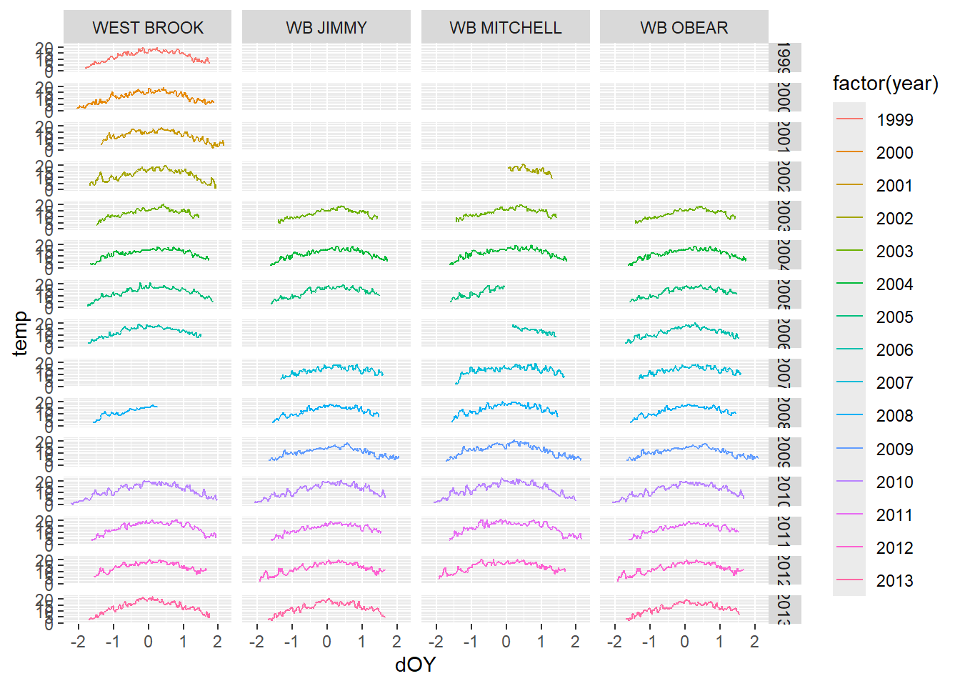
ggplot(tempDataSyncS,aes(dOY,flowLS))+
  geom_line(aes(color=factor(year)))+
  facet_grid(year~riverOrdered)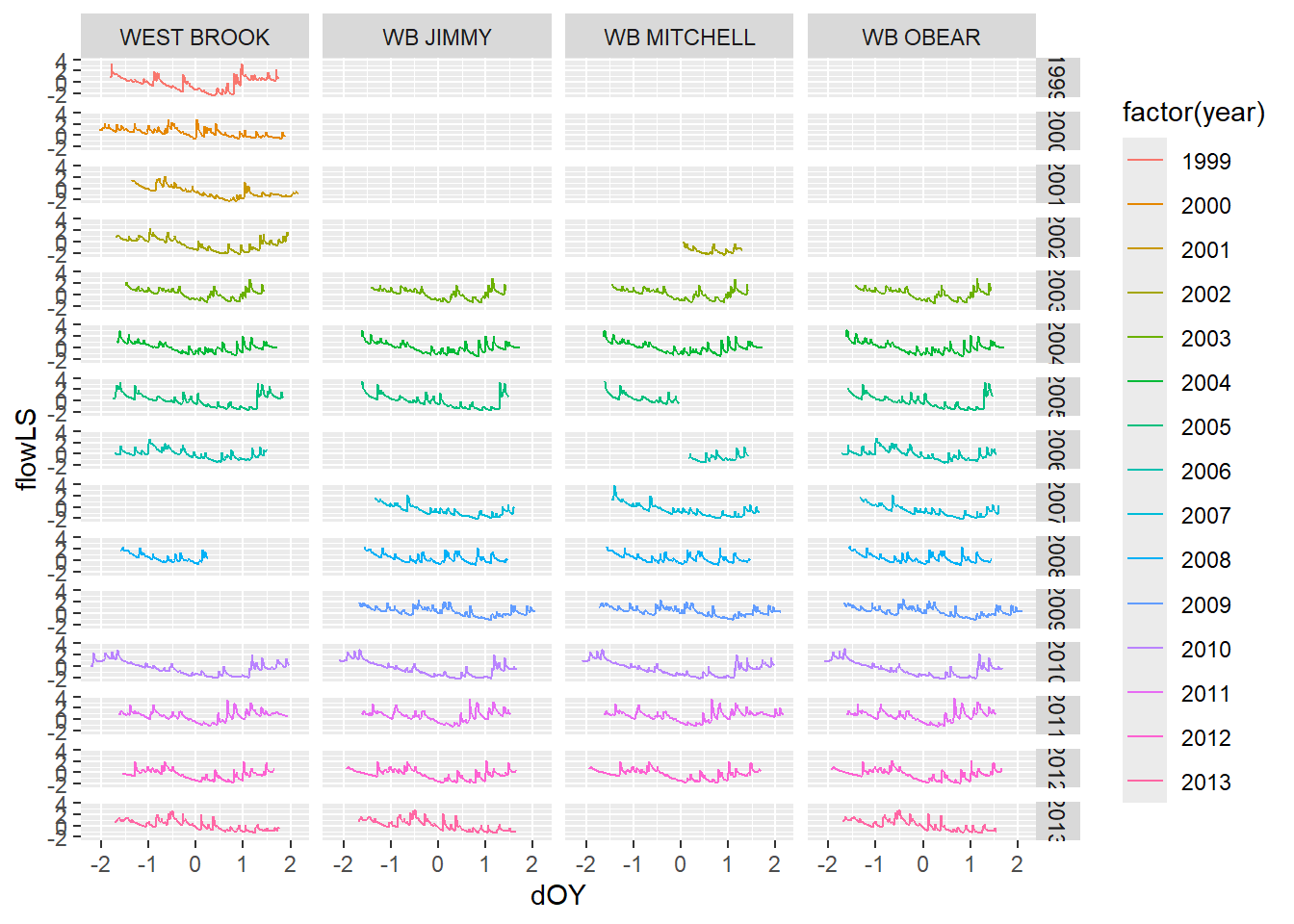
tempDataSyncS %>% ggplot(aes(x = airTemp, y = temp, color = flowLS)) + geom_point(size = 0.2) + facet_wrap(~riverOrdered) + theme_bw()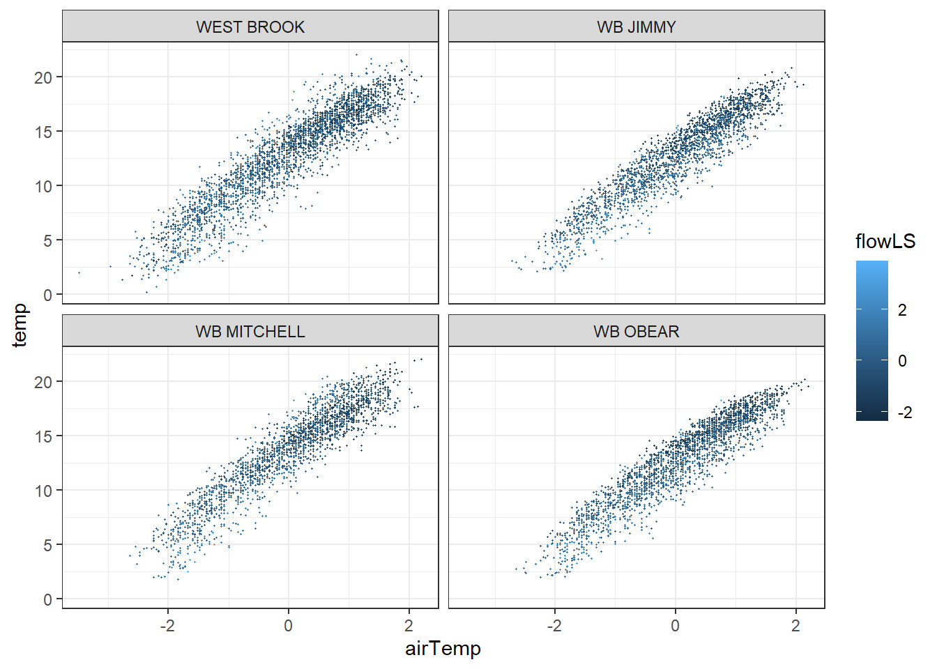
tempDataSyncS %>% ggplot(aes(x = airTemp, y = flowLS, colour = temp)) + geom_point(size = 0.2) + facet_wrap(~riverOrdered) + theme_bw() + ggpubr::stat_cor()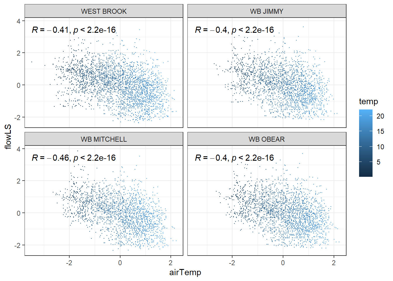
Straight from Letcher et al (2016) ::: {.cell}
cat("model {

    ###----------------- LIKELIHOOD -----------------###

    # Days without an observation on the previous day (first observation in a series)
    # No autoregressive term

    for (i in 1:nFirstObsRows){
      temp[firstObsRows[i]] ~ dnorm(stream.mu[firstObsRows[i]], pow(sigma, -2))
      stream.mu[firstObsRows[i]] <- trend[firstObsRows[i]]
      trend[firstObsRows[i]] <- inprod(B.0[], X.0[firstObsRows[i], ]) + inprod(B.year[year[firstObsRows[i]], ], X.year[firstObsRows[i], ])
      }

    # Days with an observation on the previous dat (all days following the first day)
    # Includes autoregressive term (ar1)

    for (i in 1:nEvalRows){
      temp[evalRows[i]] ~ dnorm(stream.mu[evalRows[i]], pow(sigma, -2))
      stream.mu[evalRows[i]] <- trend[evalRows[i]] + ar1[river[evalRows[i]]] * (temp[evalRows[i]-1] - trend[ evalRows[i]-1 ])
      trend[evalRows[i]]  <- inprod(B.0[], X.0[evalRows[i], ]) + inprod(B.year[year[evalRows[i]], ], X.year[evalRows[i], ])
      }


    ###----------------- PRIORS ---------------------###

    # ar1, hierarchical by site
    for (i in 1:nRiver){
      ar1[i] ~ dnorm(ar1Mean, pow(ar1SD,-2) ) T(-1,1)
    }
    ar1Mean ~ dunif( -1,1 )
    ar1SD ~ dunif( 0, 2 )

    # model variance
    sigma ~ dunif(0, 100)


    # fixed effect coefficients
    for (k in 1:K.0) {
      B.0[k] ~ dnorm(0, 0.001)
      }


    # YEAR EFFECTS
    # Priors for random effects of year
    for (t in 1:Ti) { # Ti years
      B.year[t, 1:L] ~ dmnorm(mu.year[ ], tau.B.year[ , ])
      }

    mu.year[1] <- 0

    for (l in 2:L) {
      mu.year[l] ~ dnorm(0, 0.0001)
      }

    # Prior on multivariate normal std deviation
    tau.B.year[1:L, 1:L] ~ dwish(W.year[ , ], df.year)
    df.year <- L + 1
    sigma.B.year[1:L, 1:L] <- inverse(tau.B.year[ , ])
    for (l in 1:L) {
      for (l.prime in 1:L) {
        rho.B.year[l, l.prime] <- sigma.B.year[l, l.prime]/sqrt(sigma.B.year[l, l]*sigma.B.year[l.prime, l.prime])
        }
      sigma.b.year[l] <- sqrt(sigma.B.year[l, l])
    }


    ###----------------- DERIVED VALUES -------------###
    residuals[1] <- 0 # hold the place. Not sure if this is necessary...
    for (i in 2:n) {
      residuals[i] <- temp[i] - stream.mu[i]
    }

    }", file = "JAGS models/DailyTempModelJAGS_Letcher.txt")
:::
Get first observation indices and check that nFirstRowObs equals the number of unique site-years: must be TRUE! ::: {.cell}
# row indices for first observation in each site-year
firstObsRows <- unlist(tempDataSyncS %>%
  group_by(siteYear) %>%
  summarize(index = rowNum[min(which(!is.na(temp)))]) %>%
  ungroup() %>%
  select(index))
nFirstObsRows <- length(firstObsRows)

# does the number of first observations match the number of site years?
nFirstObsRows == length(unique(tempDataSyncS$siteYear))
[1] TRUE:::
Get row indices for all other observations ::: {.cell}
evalRows <- unlist(tempDataSyncS %>% filter(!rowNum %in% firstObsRows) %>% select(rowNum))
nEvalRows <- length(evalRows)
:::
Fixed and random effect data ::: {.cell}
data.fixed <- data.frame(intercept = 1
                         ,airTemp = tempDataSyncS$airTemp
                         ,airTempLag1 = tempDataSyncS$airTempLagged1
                         ,airTempLag2 = tempDataSyncS$airTempLagged2

                         ,flow =  tempDataSyncS$flowLS

                         ,airFlow = tempDataSyncS$airTemp * tempDataSyncS$flowLS
#                         ,air1Flow = tempDataSyncS$airTempLagged1 * tempDataSyncS$flowLS
#                         ,air2Flow = tempDataSyncS$airTempLagged2 * tempDataSyncS$flowLS

                         #main river effects
                         ,river1 = tempDataSyncS$river1
                         ,river2 = tempDataSyncS$river2
                         ,river3 = tempDataSyncS$river3

                         #river interaction with air temp
                         ,river1Air = tempDataSyncS$river1 * tempDataSyncS$airTemp
                         ,river2Air = tempDataSyncS$river2 * tempDataSyncS$airTemp
                         ,river3Air = tempDataSyncS$river3 * tempDataSyncS$airTemp

                          )

data.random.years <- data.frame(intercept.year = 1,
                     dOY  = tempDataSyncS$dOY,
                     dOY2 = tempDataSyncS$dOY^2,
                     dOY3 = tempDataSyncS$dOY^3
                     )
:::
Misc. objects ::: {.cell}
Ti <- length(unique(tempDataSyncS$year))
L <- dim(data.random.years)[2]
W.year <- diag(L)
:::
Combine data in list ::: {.cell}
# combine data in a list
jags.data <- list("temp" = tempDataSyncS$temp,
                  "nFirstObsRows" = nFirstObsRows,
                  "firstObsRows" = firstObsRows,
                  "nEvalRows" = nEvalRows,
                  "evalRows" = evalRows,
                  "X.0" = data.fixed,
                  "X.year" = data.random.years,
                  "K.0" = dim(data.fixed)[2],
                  "nRiver" = length(unique(tempDataSyncS$site)),
                  "Ti" = Ti,
                  "L" = L,
                  "W.year" = W.year,
                  "n" = dim(tempDataSyncS)[1],
                  "year" = as.factor(tempDataSyncS$year),
                  "river" = as.factor(tempDataSyncS$riverOrdered)
                  )
:::
Parameters to monitor ::: {.cell}
jags.params <- c("residuals",
            "deviance",
 #           "pD",
            "sigma",
            "B.0",
            "B.year",
            "rho.B.year",
            "mu.year",
            "sigma.b.year",
            "stream.mu",
            "ar1" ,
            "ar1Mean",
            "ar1SD",
            "temp"
            )
:::
fit0 <- jags.parallel(data = jags.data, inits = NULL, parameters.to.save = jags.params, model.file = "JAGS models/DailyTempModelJAGS_Letcher.txt",
            n.chains = 10, n.thin = 5, n.burnin = 500, n.iter = 1500, DIC = TRUE)
beep()Save to file ::: {.cell}
saveRDS(fit0, "Model objects/LetcherTempModel_PeerJ2016.RDS"):::
Read in fitted model object ::: {.cell}
fit0 <- readRDS("Model objects/LetcherTempModel_PeerJ2016.RDS"):::
Get MCMC samples and summary ::: {.cell}
top_mod <- fit0
# generate MCMC samples and store as an array
modelout <- top_mod$BUGSoutput
McmcList <- vector("list", length = dim(modelout$sims.array)[2])
for(i in 1:length(McmcList)) { McmcList[[i]] = as.mcmc(modelout$sims.array[,i,]) }
# rbind MCMC samples from 10 chains
Mcmcdat <- rbind(McmcList[[1]], McmcList[[2]], McmcList[[3]], McmcList[[4]], McmcList[[5]], McmcList[[6]], McmcList[[7]], McmcList[[8]], McmcList[[9]], McmcList[[10]])
param.summary <- modelout$summary
head(param.summary)
mean sd 2.5% 25% 50% 75%
B.0[1] 15.0942825 0.17271642 14.7510778 14.9831293 15.0931367 15.2073322
B.0[2] 1.5201578 0.02723257 1.4673158 1.5016734 1.5199031 1.5390533
B.0[3] 0.1955279 0.01619090 0.1631752 0.1845110 0.1954986 0.2069212
B.0[4] 0.1545523 0.01642121 0.1208057 0.1442824 0.1542702 0.1647775
B.0[5] 0.3629916 0.01520228 0.3334788 0.3523900 0.3635001 0.3730769
B.0[6] -0.1292206 0.01180889 -0.1523336 -0.1368216 -0.1290627 -0.1214532
97.5% Rhat n.eff
B.0[1] 15.4398786 1.0038273 1000
B.0[2] 1.5732813 1.0034739 1100
B.0[3] 0.2254210 0.9999951 2000
B.0[4] 0.1871898 1.0028484 1300
B.0[5] 0.3919732 1.0006563 2000
B.0[6] -0.1065415 0.9998802 2000:::
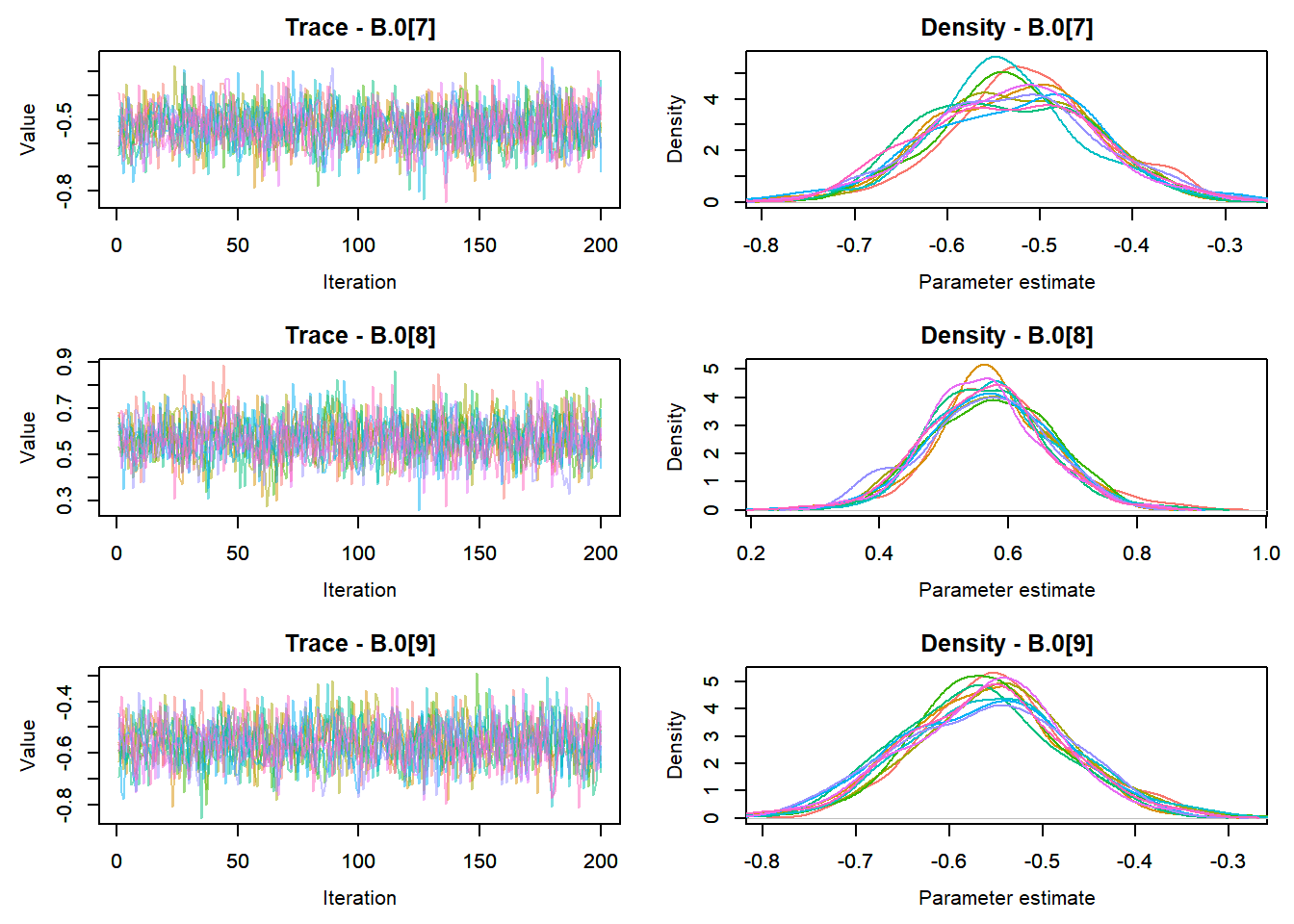
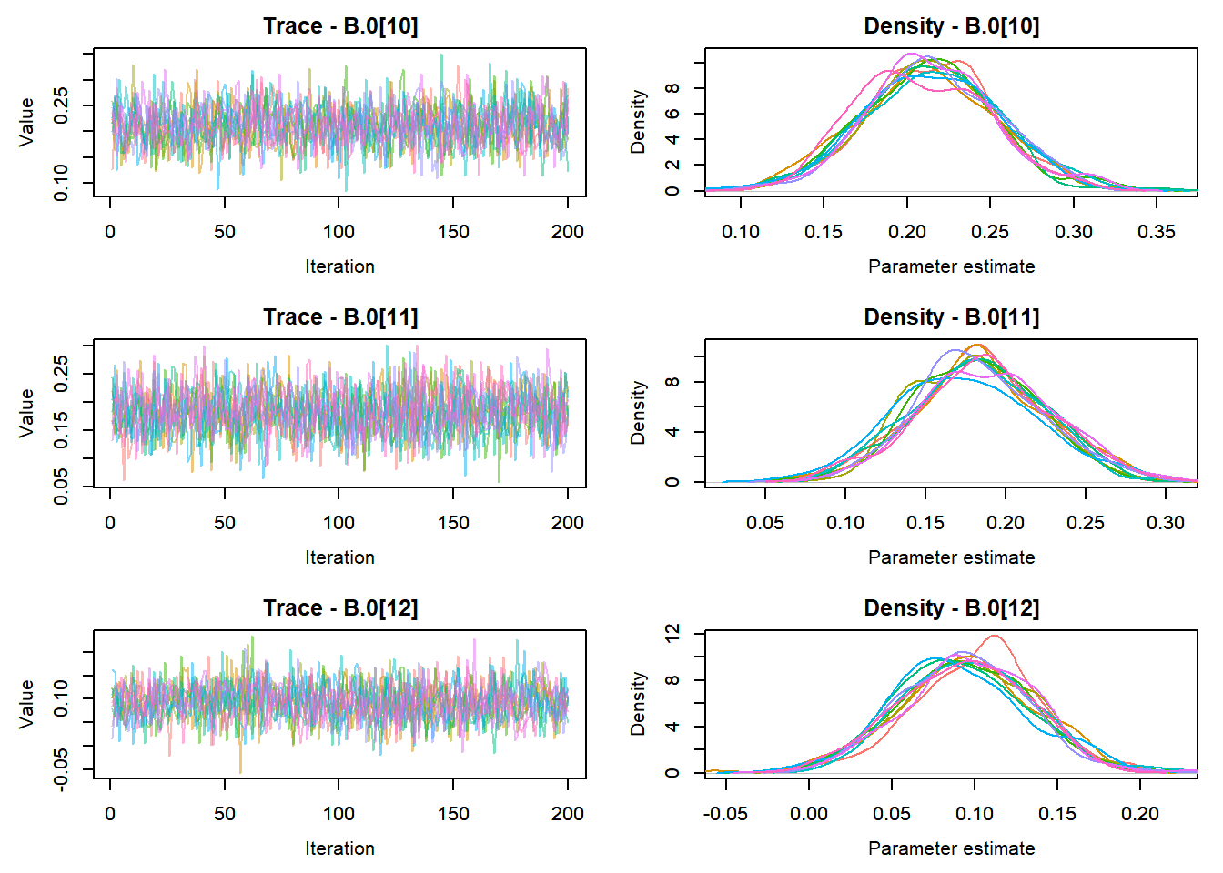
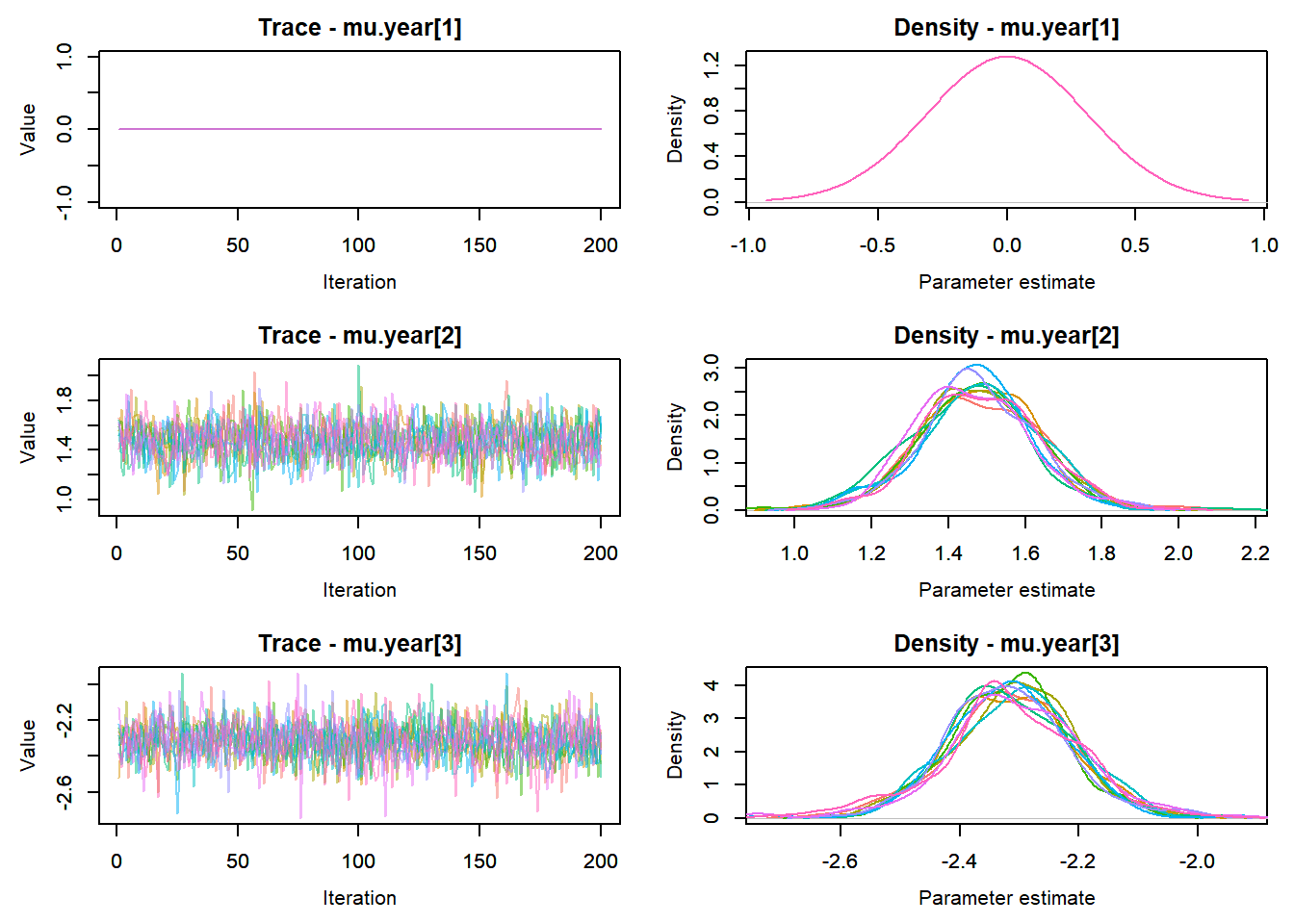
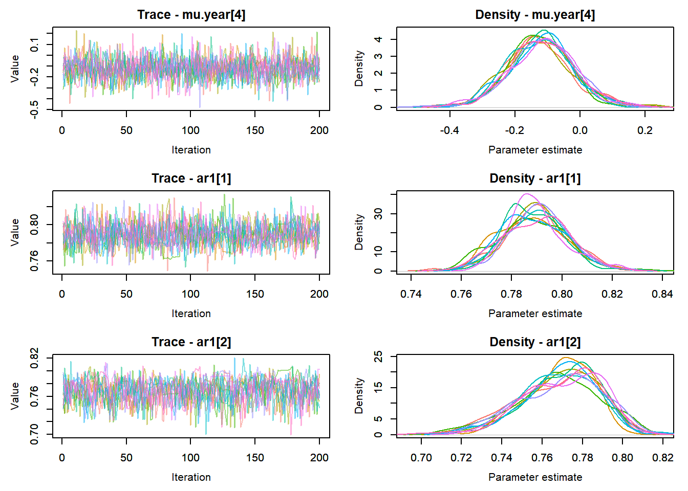
Any problematic R-hat values (>1.05)? ::: {.cell}
top_mod$BUGSoutput$summary[,8][top_mod$BUGSoutput$summary[,8] > 1.05]named numeric(0):::
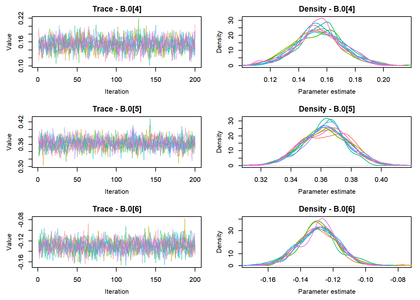
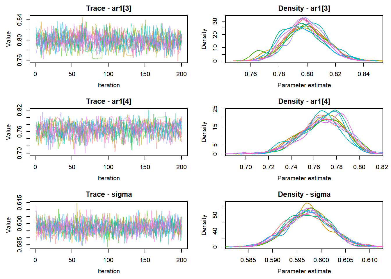
View traceplots ::: {.cell}
MCMCtrace(top_mod, ind = TRUE,
          params = c("B.0", "mu.year",
                     "ar1",
                     "sigma"), pdf = FALSE)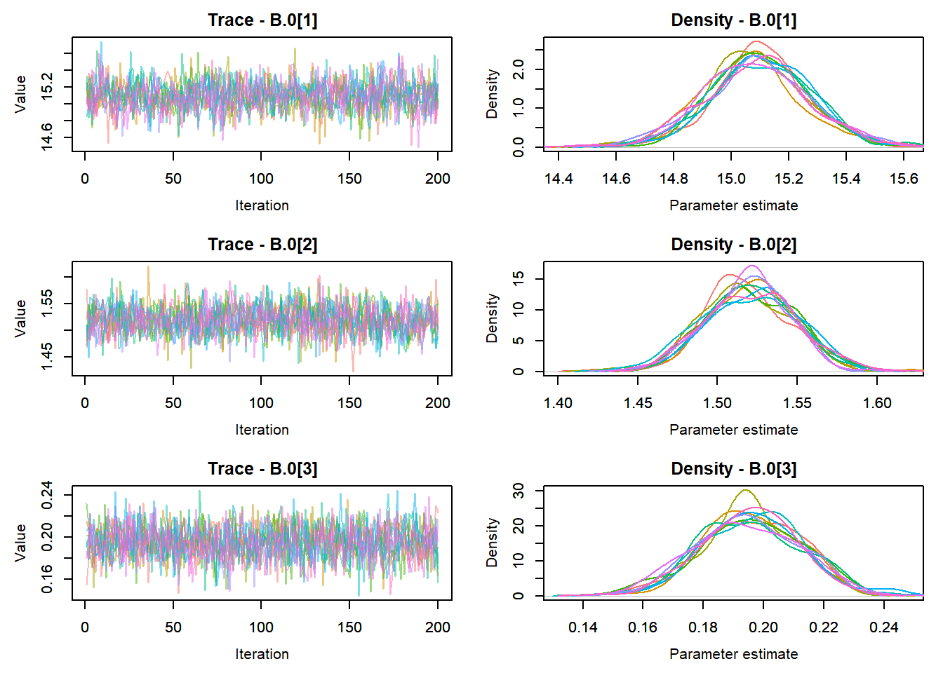
:::
Convert to ggs object ::: {.cell}
ggfit <- ggs(as.mcmc(top_mod), keep_original_order = TRUE)
head(ggfit)
# A tibble: 6 × 4
Iteration Chain Parameter value
<int> <int> <fct> <dbl>
1 1 1 ar1[1] 0.773
2 2 1 ar1[1] 0.799
3 3 1 ar1[1] 0.817
4 4 1 ar1[1] 0.796
5 5 1 ar1[1] 0.811
6 6 1 ar1[1] 0.801:::
Format observed and predicted values ::: {.cell}
Mcmcdat <- as_tibble(Mcmcdat)

# subset expected and observed MCMC samples
ppdat_exp <- as.matrix(Mcmcdat[,startsWith(names(Mcmcdat), "stream.mu[")])
ppdat_obs <- as.matrix(Mcmcdat[,startsWith(names(Mcmcdat), "temp[")])
:::
Bayesian p-value ::: {.cell}
sum(ppdat_exp > ppdat_obs) / (dim(ppdat_obs)[1]*dim(ppdat_obs)[2])[1] 0.4975728:::
PP-check, global ::: {.cell}
ppdat_obs_mean <- apply(ppdat_obs, 2, mean)
ppdat_exp_mean <- apply(ppdat_exp, 2, mean)
tibble(obs = ppdat_obs_mean, exp = ppdat_exp_mean) %>%
  ggplot(aes(x = obs, y = exp)) +
  geom_point(alpha = 0.1) +
  # geom_smooth(method = "lm") +
  geom_abline(intercept = 0, slope = 1, color = "red") +
  theme_bw() + theme(panel.grid = element_blank()) +
  xlab("Observed") + ylab("Predicted (mean)")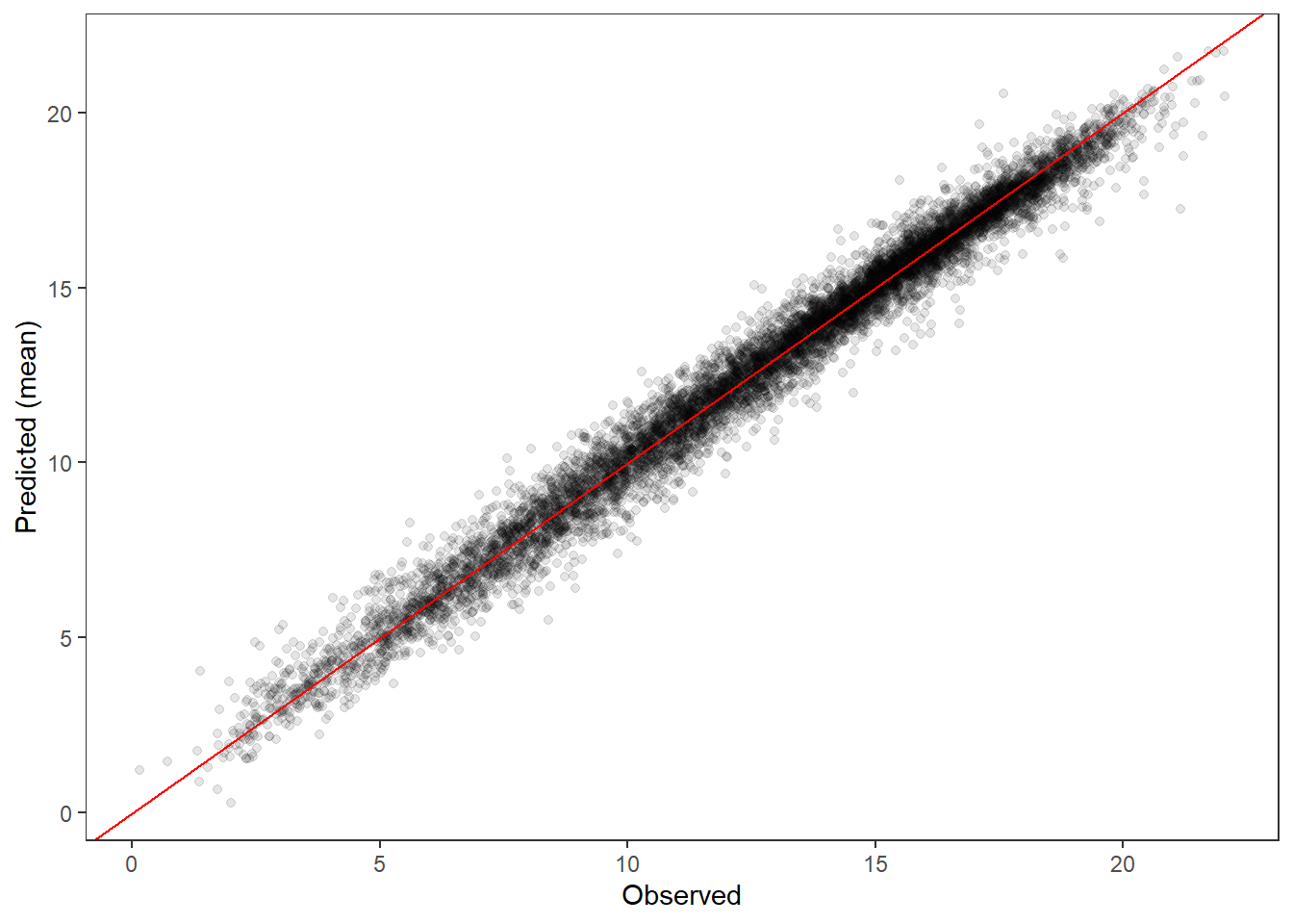
:::
PP-check by river and year ::: {.cell}
tibble(obs = ppdat_obs_mean, exp = ppdat_exp_mean, river = tempDataSyncS$riverOrdered, year = tempDataSyncS$year) %>%
  ggplot(aes(x = obs, y = exp)) +
  geom_point(alpha = 0.1) +
  # geom_smooth(method = "lm") +
  geom_abline(intercept = 0, slope = 1, color = "red") +
  theme_bw() + theme(panel.grid = element_blank()) +
  xlab("Observed") + ylab("Predicted (mean)") +
  facet_grid(year ~ river)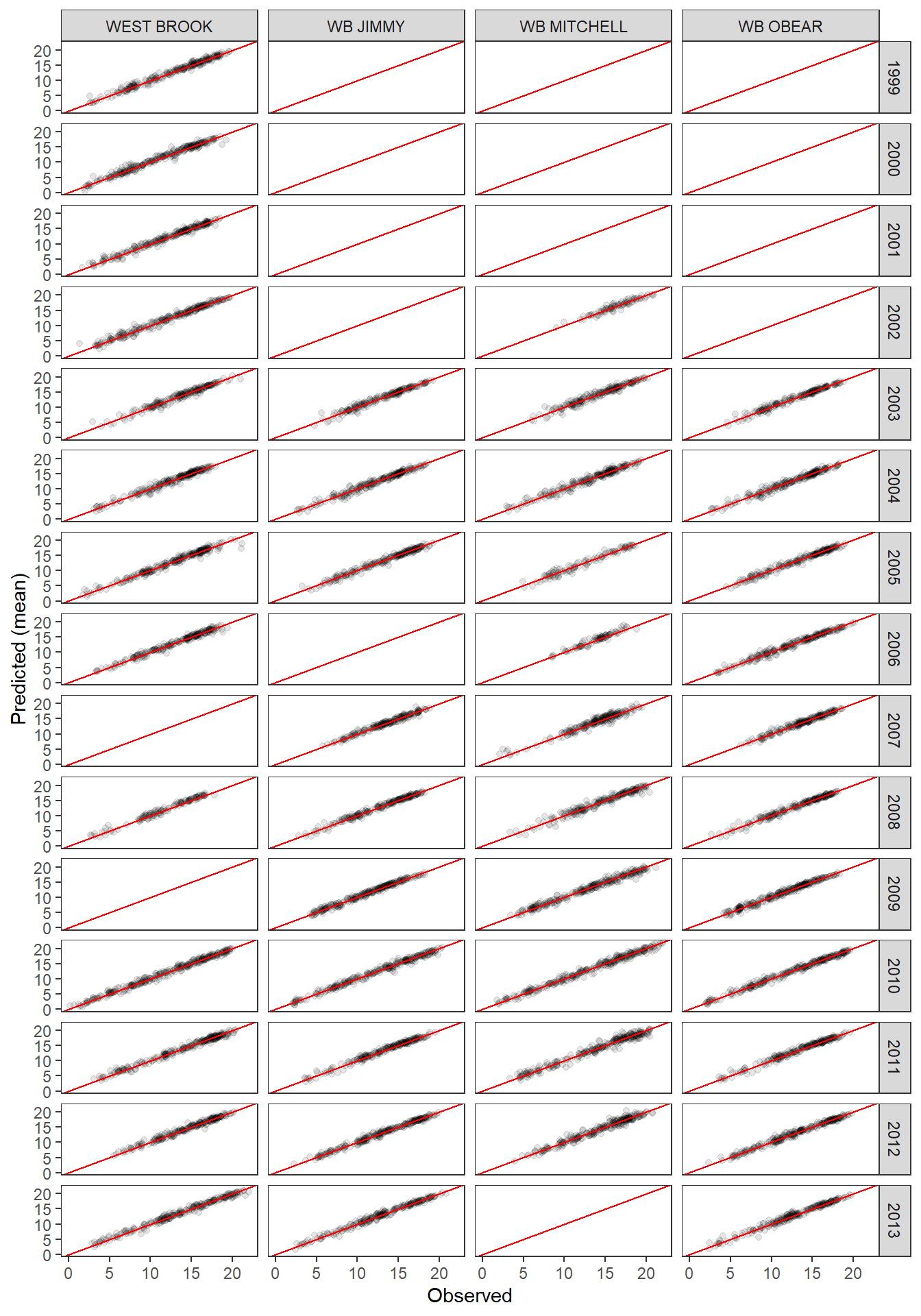
:::
Output is identical to Letcher et al. (2016), as expected
ggs_caterpillar(ggfit %>% filter(Parameter == "B.0[1]"), sort = FALSE) + scale_y_discrete(labels = "Intercept") + theme_bw()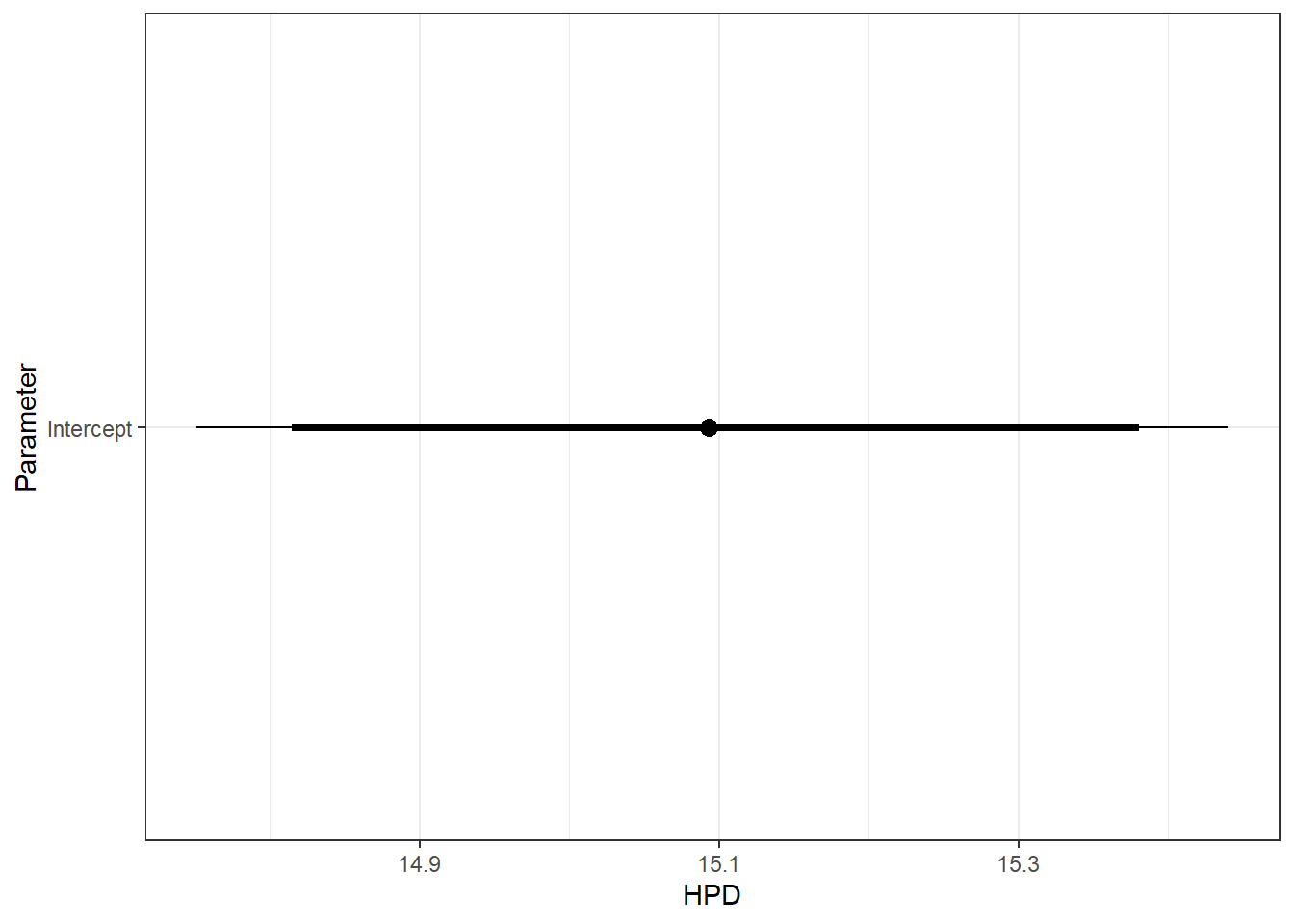
ggs_caterpillar(ggfit %>% filter(Parameter %in% grep("B.0", unique(ggfit$Parameter), value = TRUE)[-1]) %>%
                  mutate(Parameter = factor(Parameter, levels = c("B.0[2]", "B.0[3]", "B.0[4]", "B.0[5]", "B.0[6]",
                                                                  "B.0[7]", "B.0[8]", "B.0[9]", "B.0[10]", "B.0[11]", "B.0[12]"))),
                sort = FALSE) + scale_y_discrete(labels = rev(c("T", "T(d-1)", "T(d-2)", "F", "T*F", "OL", "OS", "IS", "OL*T", "OS*T", "IS*T")), limits = rev) + theme_bw() + geom_vline(xintercept = 0, linetype = "dashed")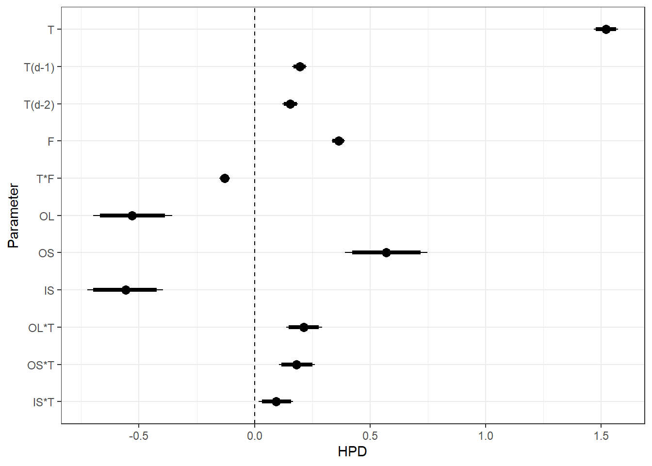
ggs_caterpillar(ggfit %>% filter(Parameter %in% grep("ar1", unique(ggfit$Parameter), value = TRUE)) %>%
                  mutate(Parameter = factor(Parameter, levels = c("ar1Mean", "ar1SD", "ar1[1]", "ar1[2]", "ar1[3]", "ar1[4]"))),
                sort = FALSE) + scale_y_discrete(labels = rev(c("ar1Mean", "ar1SD", "ar1[WB]", "ar1[OL]", "ar1[OS]", "ar1[IL]")), limits = rev) + theme_bw() + xlim(0,1)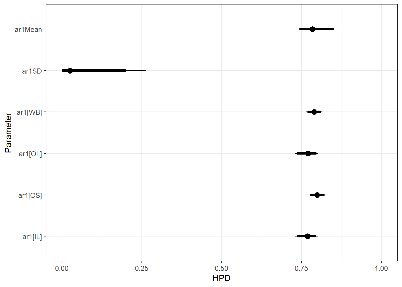
ggs_caterpillar(ggfit, family = "mu.year", sort = FALSE) + scale_y_discrete(labels = rev(c("Intercept", "Linear", "Quadratic", "Cubic")), limits = rev) + theme_bw()
ggfit %>%
  filter(Parameter %in% c("B.0[1]", "B.0[7]", "B.0[8]", "B.0[9]")) %>%
  spread(key = Parameter, value = value) %>%
  rename(int_WB = 3, os_OL = 4, os_OS = 5, os_IS = 6) %>%
  mutate(int_OL = int_WB + os_OL,
         int_OS = int_WB + os_OS,
         int_IS = int_WB + os_IS) %>%
  select(-c(os_OL, os_OS, os_IS)) %>%
  gather(int_WB:int_IS, key = "Parameter", value = "value") %>%
  mutate(Parameter = factor(Parameter, levels = c("int_WB", "int_OL", "int_OS", "int_IS"))) %>%
  ggs_caterpillar(sort = FALSE) +
  scale_y_discrete(limits = rev) +
  ylab("Intercepts") +
  theme_bw()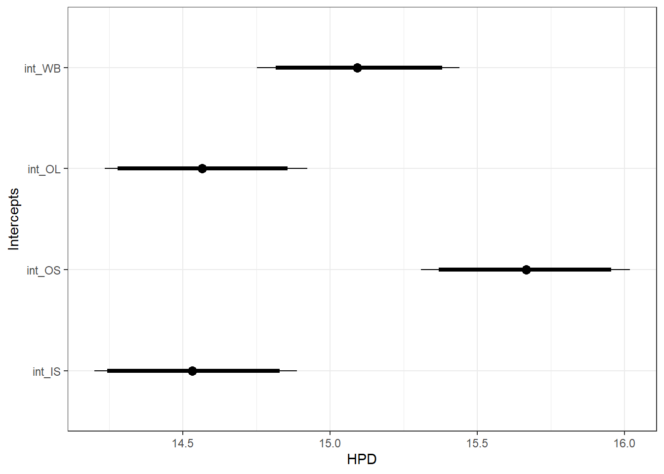
ggfit %>%
  filter(Parameter %in% c("B.0[2]", "B.0[10]", "B.0[11]", "B.0[12]")) %>%
  spread(key = Parameter, value = value) %>%
  rename(slo_WB = 6, os_OL = 3, os_OS = 4, os_IS = 5) %>%
  mutate(slo_OL = slo_WB + os_OL,
         slo_OS = slo_WB + os_OS,
         slo_IS = slo_WB + os_IS) %>%
  select(-c(os_OL, os_OS, os_IS)) %>%
  gather(slo_WB:slo_IS, key = "Parameter", value = "value") %>%
  mutate(Parameter = factor(Parameter, levels = c("slo_WB", "slo_OL", "slo_OS", "slo_IS"))) %>%
  ggs_caterpillar(sort = FALSE) +
  scale_y_discrete(limits = rev) +
  ylab("Slopes, temperature effect") +
  theme_bw()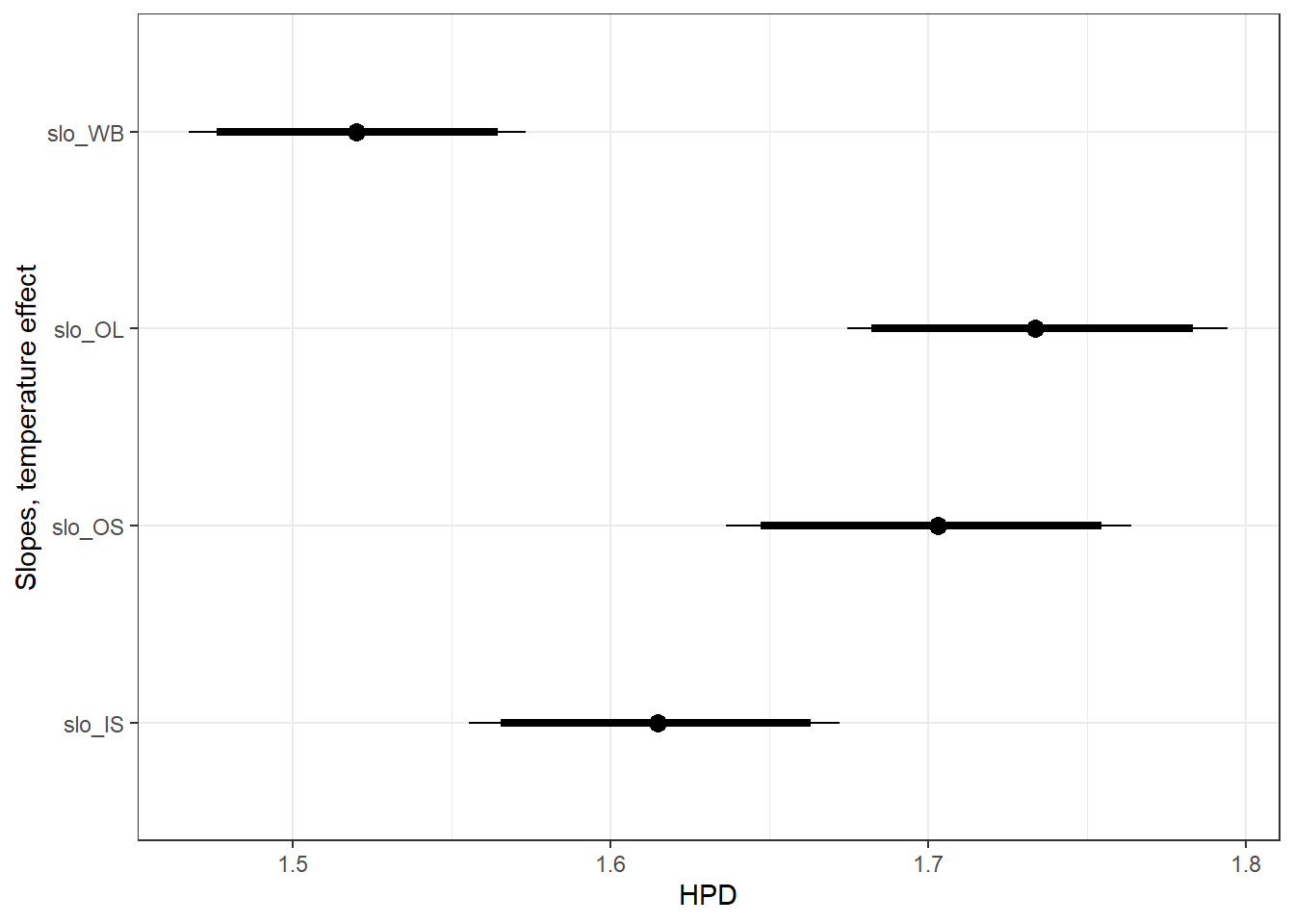
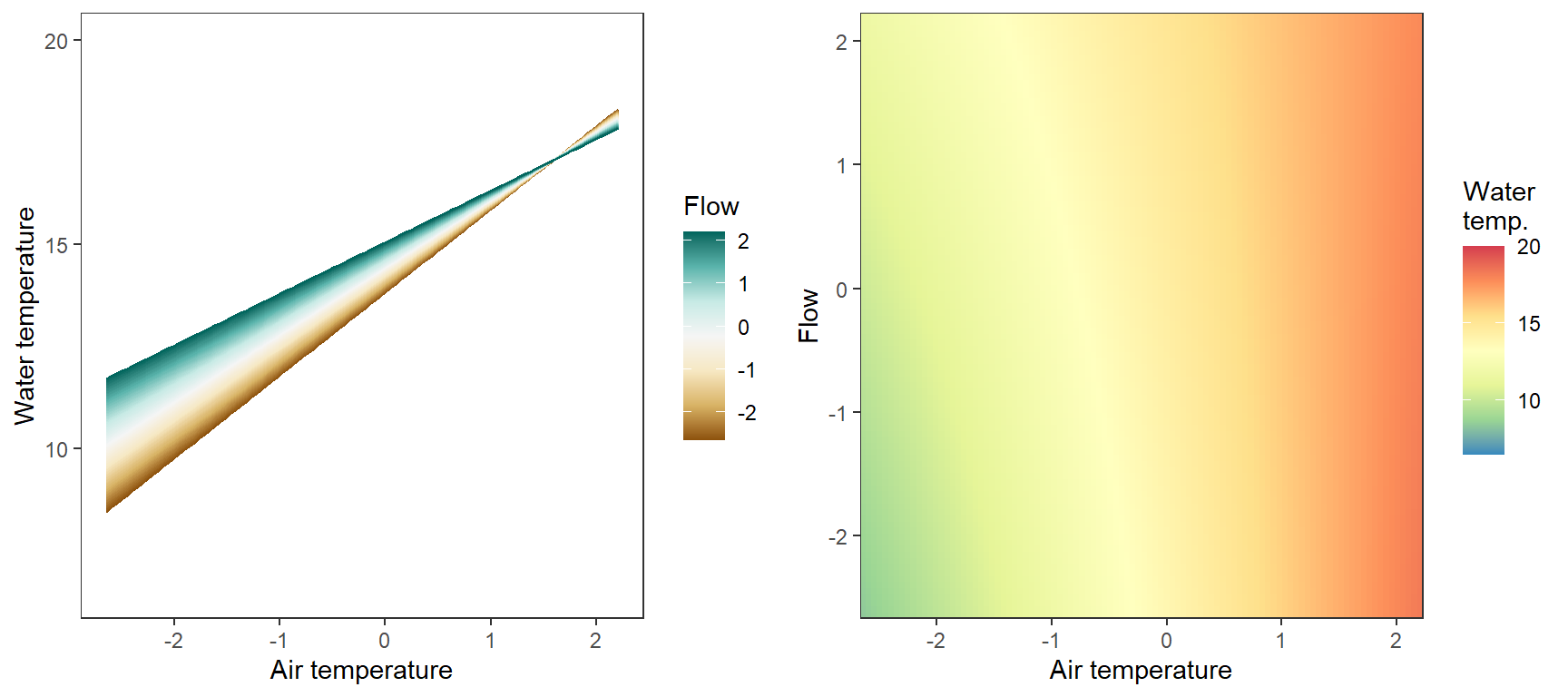
Marginal effects of air temperature x flow interaction, not accounting for lagged temperature effects, temporal autocorrelation,
# set up
np <- 100
myriv <- "WEST BROOK"
x_temp <- seq(from = min(tempDataSyncS$airTemp[tempDataSyncS$riverOrdered == myriv]),
              to = max(tempDataSyncS$airTemp[tempDataSyncS$riverOrdered == myriv]),
              length.out = np)
x_flow <- seq(from = min(tempDataSyncS$flowLS[tempDataSyncS$riverOrdered == myriv]),
              to = max(tempDataSyncS$flowLS[tempDataSyncS$riverOrdered == myriv]),
              length.out = np)
pred_df <- expand_grid(x_temp, x_flow)

# predict from model
pred_df$pred <- param.summary["B.0[1]",1] + param.summary["B.0[2]",1]*pred_df$x_temp + param.summary["B.0[5]",1]*pred_df$x_flow + param.summary["B.0[6]",1]*pred_df$x_temp*pred_df$x_flow

# lines
p1 <- ggplot(pred_df, aes(x = x_temp, y = pred, color = x_flow, group = x_flow)) +
  geom_line() +
  scale_color_distiller(palette = "BrBG", direction = +1) +
  theme_bw() + theme(panel.grid = element_blank()) +
  labs(color = "Flow") + xlab("Air temperature") + ylab("Water temperature") + ylim(6.5,20)
# heatmap
p2 <- ggplot(pred_df, aes(x = x_temp, y = x_flow)) +
  geom_tile(aes(fill = pred)) +
  scale_fill_distiller(palette = "Spectral", limits = c(6.5,20)) +
  theme_bw() + theme(panel.grid = element_blank()) +
  scale_x_continuous(expand = c(0,0)) + scale_y_continuous(expand = c(0,0)) +
  labs(fill = "Water\ntemp.") + xlab("Air temperature") + ylab("Flow") #+
  #geom_point(data = tempDataSyncS %>% filter(riverOrdered == myriv), aes(x = airTemp, y = flowLS, color = temp)) +
  #scale_color_distiller(palette = "Spectral", limits = c(0,23))
# combine
egg::ggarrange(p1, p2, nrow = 1)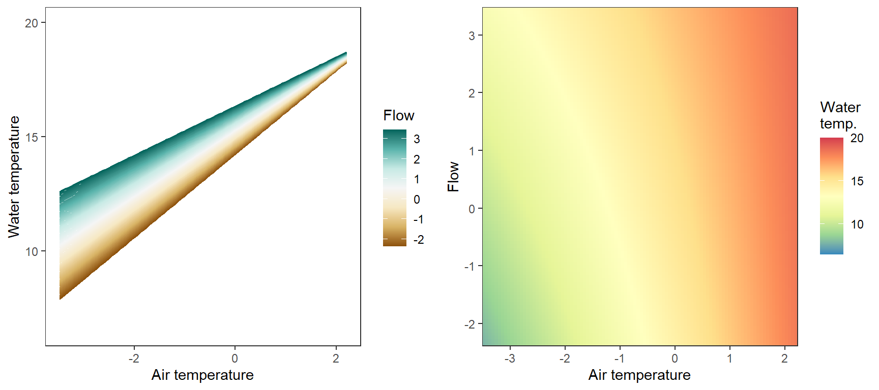
# set up
np <- 100
myriv <- "WB JIMMY"
x_temp <- seq(from = min(tempDataSyncS$airTemp[tempDataSyncS$riverOrdered == myriv]),
              to = max(tempDataSyncS$airTemp[tempDataSyncS$riverOrdered == myriv]),
              length.out = np)
x_flow <- seq(from = min(tempDataSyncS$airTemp[tempDataSyncS$riverOrdered == myriv]),
              to = max(tempDataSyncS$airTemp[tempDataSyncS$riverOrdered == myriv]),
              length.out = np)
pred_df <- expand_grid(x_temp, x_flow)

# predict from model
pred_df$pred <- param.summary["B.0[1]",1] + param.summary["B.0[2]",1]*pred_df$x_temp + param.summary["B.0[5]",1]*pred_df$x_flow + param.summary["B.0[6]",1]*pred_df$x_temp*pred_df$x_flow + param.summary["B.0[7]",1] + param.summary["B.0[10]",1]*pred_df$x_temp

# lines
p1 <- ggplot(pred_df, aes(x = x_temp, y = pred, color = x_flow, group = x_flow)) +
  geom_line() +
  scale_color_distiller(palette = "BrBG", direction = +1) +
  theme_bw() + theme(panel.grid = element_blank()) +
  labs(color = "Flow") + xlab("Air temperature") + ylab("Water temperature") + ylim(6.5,20)
# heatmap
p2 <- ggplot(pred_df, aes(x = x_temp, y = x_flow)) +
  geom_tile(aes(fill = pred)) +
  scale_fill_distiller(palette = "Spectral", limits = c(6.5,20)) +
  theme_bw() + theme(panel.grid = element_blank()) +
  scale_x_continuous(expand = c(0,0)) + scale_y_continuous(expand = c(0,0)) +
  labs(fill = "Water\ntemp.") + xlab("Air temperature") + ylab("Flow")
# combine
egg::ggarrange(p1, p2, nrow = 1)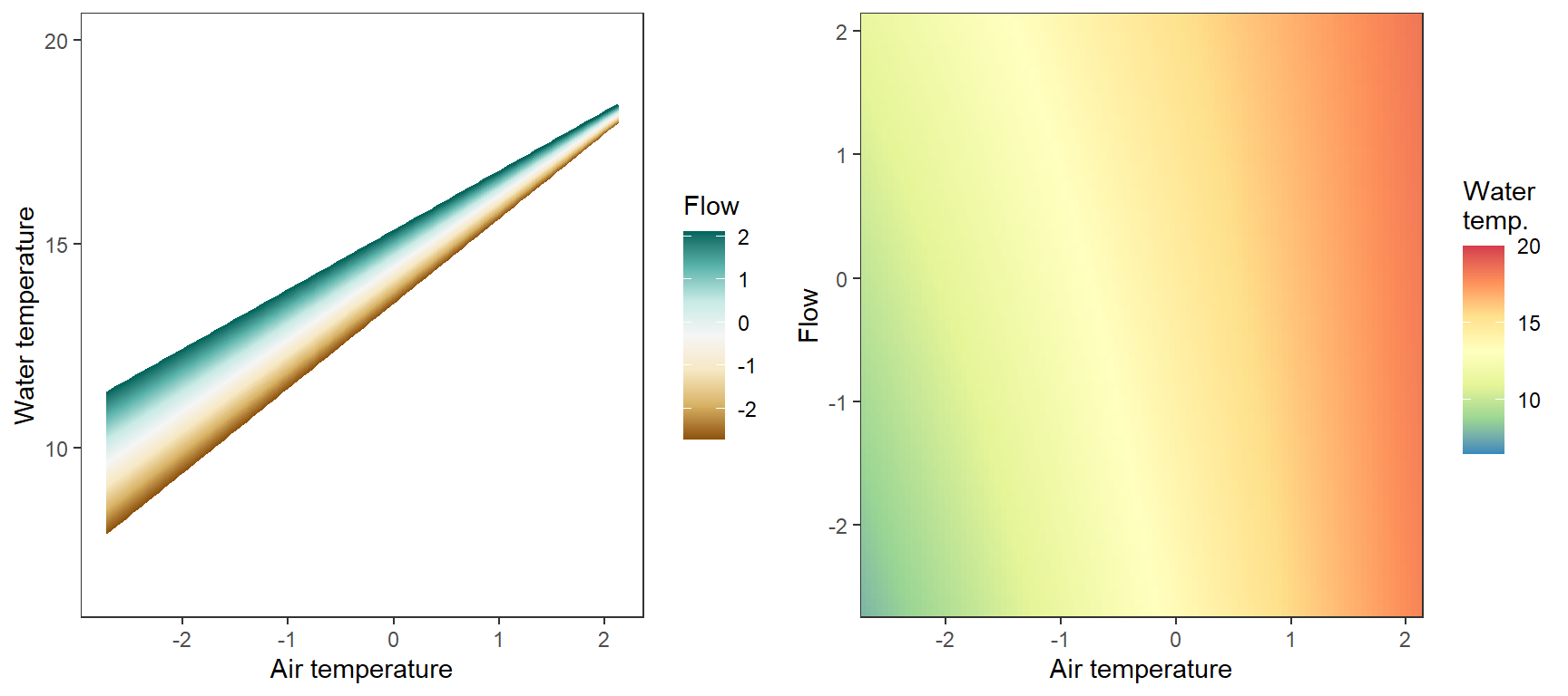
# set up
np <- 100
myriv <- "WB MITCHELL"
x_temp <- seq(from = min(tempDataSyncS$airTemp[tempDataSyncS$riverOrdered == myriv]),
              to = max(tempDataSyncS$airTemp[tempDataSyncS$riverOrdered == myriv]),
              length.out = np)
x_flow <- seq(from = min(tempDataSyncS$airTemp[tempDataSyncS$riverOrdered == myriv]),
              to = max(tempDataSyncS$airTemp[tempDataSyncS$riverOrdered == myriv]),
              length.out = np)
pred_df <- expand_grid(x_temp, x_flow)

# predict from model
pred_df$pred <- param.summary["B.0[1]",1] + param.summary["B.0[2]",1]*pred_df$x_temp + param.summary["B.0[5]",1]*pred_df$x_flow + param.summary["B.0[6]",1]*pred_df$x_temp*pred_df$x_flow + param.summary["B.0[8]",1] + param.summary["B.0[11]",1]*pred_df$x_temp

# lines
p1 <- ggplot(pred_df, aes(x = x_temp, y = pred, color = x_flow, group = x_flow)) +
  geom_line() +
  scale_color_distiller(palette = "BrBG", direction = +1) +
  theme_bw() + theme(panel.grid = element_blank()) +
  labs(color = "Flow") + xlab("Air temperature") + ylab("Water temperature") + ylim(6.5,20)
# heatmap
p2 <- ggplot(pred_df, aes(x = x_temp, y = x_flow)) +
  geom_tile(aes(fill = pred)) +
  scale_fill_distiller(palette = "Spectral", limits = c(6.5,20)) +
  theme_bw() + theme(panel.grid = element_blank()) +
  scale_x_continuous(expand = c(0,0)) + scale_y_continuous(expand = c(0,0)) +
  labs(fill = "Water\ntemp.") + xlab("Air temperature") + ylab("Flow")
# combine
egg::ggarrange(p1, p2, nrow = 1)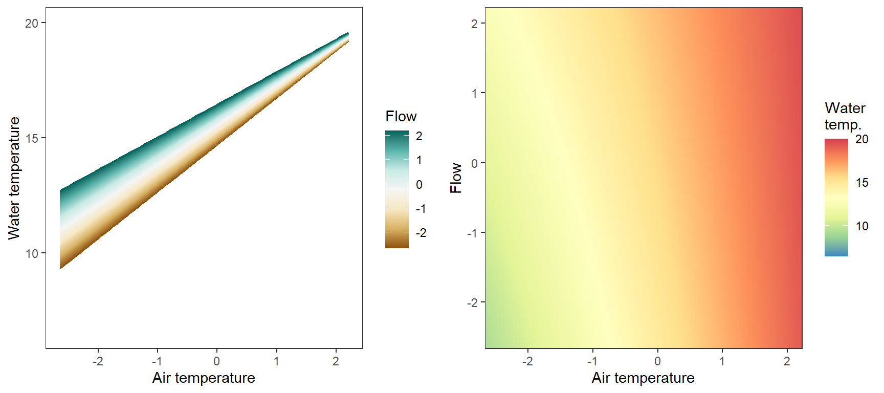
# set up
np <- 100
myriv <- "WB OBEAR"
x_temp <- seq(from = min(tempDataSyncS$airTemp[tempDataSyncS$riverOrdered == myriv]),
              to = max(tempDataSyncS$airTemp[tempDataSyncS$riverOrdered == myriv]),
              length.out = np)
x_flow <- seq(from = min(tempDataSyncS$airTemp[tempDataSyncS$riverOrdered == myriv]),
              to = max(tempDataSyncS$airTemp[tempDataSyncS$riverOrdered == myriv]),
              length.out = np)
pred_df <- expand_grid(x_temp, x_flow)

# predict from model
pred_df$pred <- param.summary["B.0[1]",1] + param.summary["B.0[2]",1]*pred_df$x_temp + param.summary["B.0[5]",1]*pred_df$x_flow + param.summary["B.0[6]",1]*pred_df$x_temp*pred_df$x_flow + param.summary["B.0[9]",1] + param.summary["B.0[12]",1]*pred_df$x_temp

# lines
p1 <- ggplot(pred_df, aes(x = x_temp, y = pred, color = x_flow, group = x_flow)) +
  geom_line() +
  scale_color_distiller(palette = "BrBG", direction = +1) +
  theme_bw() + theme(panel.grid = element_blank()) +
  labs(color = "Flow") + xlab("Air temperature") + ylab("Water temperature") + ylim(6.5,20)
# heatmap
p2 <- ggplot(pred_df, aes(x = x_temp, y = x_flow)) +
  geom_tile(aes(fill = pred)) +
  scale_fill_distiller(palette = "Spectral", limits = c(6.5,20)) +
  theme_bw() + theme(panel.grid = element_blank()) +
  scale_x_continuous(expand = c(0,0)) + scale_y_continuous(expand = c(0,0)) +
  labs(fill = "Water\ntemp.") + xlab("Air temperature") + ylab("Flow")
# combine
egg::ggarrange(p1, p2, nrow = 1)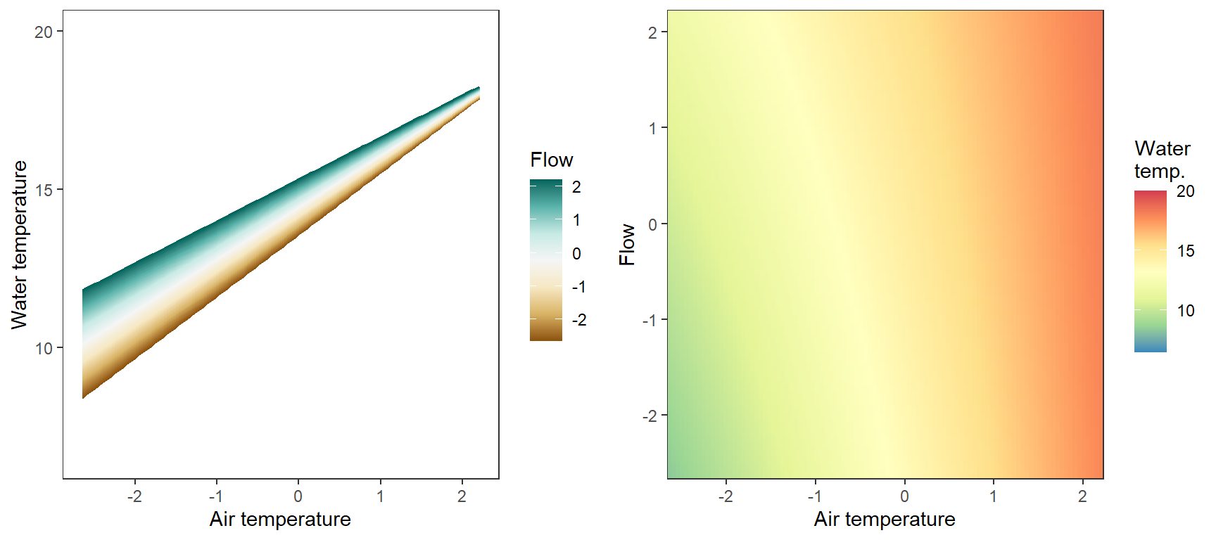
Fit the same model as above, but draw the intercepts and temperature effects hierarchically and check that the output matches
Modify Letcher model to estimate intercepts and slopes hierarchically ::: {.cell}
cat("model {

    ###----------------- LIKELIHOOD -----------------###

    # Days without an observation on the previous day (first observation in a series)
    # No autoregressive term

    for (i in 1:nFirstObsRows){
      temp[firstObsRows[i]] ~ dnorm(stream.mu[firstObsRows[i]], pow(sigma, -2))
      stream.mu[firstObsRows[i]] <- trend[firstObsRows[i]]
      trend[firstObsRows[i]] <- inprod(B.0[], X.0[firstObsRows[i], ]) +
                                inprod(B.site[site[firstObsRows[i]], ], X.site[firstObsRows[i], ]) +
                                inprod(B.year[year[firstObsRows[i]], ], X.year[firstObsRows[i], ])

      }

    # Days with an observation on the previous dat (all days following the first day)
    # Includes autoregressive term (ar1)

    for (i in 1:nEvalRows){
      temp[evalRows[i]] ~ dnorm(stream.mu[evalRows[i]], pow(sigma, -2))
      stream.mu[evalRows[i]] <- trend[evalRows[i]] + ar1[site[evalRows[i]]] * (temp[evalRows[i]-1] - trend[ evalRows[i]-1 ])
      trend[evalRows[i]] <- inprod(B.0[], X.0[evalRows[i], ]) +
                            inprod(B.site[site[evalRows[i]], ], X.site[evalRows[i], ]) +
                            inprod(B.year[year[evalRows[i]], ], X.year[evalRows[i], ])
      }


    ###----------------- PRIORS ---------------------###

    # ar1, hierarchical by site
    for (i in 1:nsites){
      ar1[i] ~ dnorm(ar1Mean, pow(ar1SD,-2) ) T(-1,1)
    }
    ar1Mean ~ dunif( -1,1 )
    ar1SD ~ dunif( 0, 2 )

    # model variance
    sigma ~ dunif(0, 100)


    # fixed effect coefficients
    for (k in 1:Kfixed) {
      B.0[k] ~ dnorm(0, 0.001)
      }

    # random effect coefficients (by site)
    for (k in 1:Krandom) {
      sigma.B.site[k] ~ dunif(0, 100)
      for (i in 1:nsites) {
        B.site[i,k] ~ dnorm(0, pow(sigma.B.site[k], -2))
      }
    }

    # YEAR EFFECTS
    # Priors for random effects of year
    for (t in 1:Ti) { # Ti years
      B.year[t, 1:L] ~ dmnorm(mu.year[ ], tau.B.year[ , ])
      }

    mu.year[1] <- 0

    for (l in 2:L) {
      mu.year[l] ~ dnorm(0, 0.0001)
      }

    # Prior on multivariate normal std deviation
    tau.B.year[1:L, 1:L] ~ dwish(W.year[ , ], df.year)
    df.year <- L + 1
    sigma.B.year[1:L, 1:L] <- inverse(tau.B.year[ , ])
    for (l in 1:L) {
      for (l.prime in 1:L) {
        rho.B.year[l, l.prime] <- sigma.B.year[l, l.prime]/sqrt(sigma.B.year[l, l]*sigma.B.year[l.prime, l.prime])
        }
      sigma.b.year[l] <- sqrt(sigma.B.year[l, l])
    }


    ###----------------- DERIVED VALUES -------------###
    residuals[1] <- 0 # hold the place. Not sure if this is necessary...
    for (i in 2:n) {
      residuals[i] <- temp[i] - stream.mu[i]
    }

    }", file = "JAGS models/DailyTempModelJAGS_Letcher_hierarchical.txt")
:::
Get first observation indices and check that nFirstRowObs equals the number of unique site-years: must be TRUE! ::: {.cell}
# row indices for first observation in each site-year
firstObsRows <- unlist(tempDataSyncS %>%
  group_by(siteYear) %>%
  summarize(index = rowNum[min(which(!is.na(temp)))]) %>%
  ungroup() %>%
  select(index))
nFirstObsRows <- length(firstObsRows)

# does the number of first observations match the number of site years?
nFirstObsRows == length(unique(tempDataSyncS$siteYear))
[1] TRUE:::
Get row indices for all other observations ::: {.cell}
evalRows <- unlist(tempDataSyncS %>% filter(!rowNum %in% firstObsRows) %>% select(rowNum))
nEvalRows <- length(evalRows)
:::
Fixed and random effect data ::: {.cell}
data.random <- data.frame(intercept = 1,
                          airTemp = tempDataSyncS$airTemp )

data.fixed <- data.frame(#intercept = 1
                         #,airTemp = tempDataSyncS$airTemp
                         airTempLag1 = tempDataSyncS$airTempLagged1
                         ,airTempLag2 = tempDataSyncS$airTempLagged2

                         ,flow =  tempDataSyncS$flowLS

                         ,airFlow = tempDataSyncS$airTemp * tempDataSyncS$flowLS
#                         ,air1Flow = tempDataSyncS$airTempLagged1 * tempDataSyncS$flowLS
#                         ,air2Flow = tempDataSyncS$airTempLagged2 * tempDataSyncS$flowLS

                         #main river effects
                         # ,river1 = tempDataSyncS$river1
                         # ,river2 = tempDataSyncS$river2
                         # ,river3 = tempDataSyncS$river3
                         #
                         # #river interaction with air temp
                         # ,river1Air = tempDataSyncS$river1 * tempDataSyncS$airTemp
                         # ,river2Air = tempDataSyncS$river2 * tempDataSyncS$airTemp
                         # ,river3Air = tempDataSyncS$river3 * tempDataSyncS$airTemp

                          )

data.random.years <- data.frame(intercept.year = 1,
                     dOY  = tempDataSyncS$dOY,
                     dOY2 = tempDataSyncS$dOY^2,
                     dOY3 = tempDataSyncS$dOY^3
                     )
:::
Misc. objects ::: {.cell}
Ti <- length(unique(tempDataSyncS$year))
L <- dim(data.random.years)[2]
W.year <- diag(L)
:::
Combine data in list ::: {.cell}
# combine data in a list
jags.data <- list("temp" = tempDataSyncS$temp,
                  "nFirstObsRows" = nFirstObsRows,
                  "firstObsRows" = firstObsRows,
                  "nEvalRows" = nEvalRows,
                  "evalRows" = evalRows,
                  "X.0" = as.matrix(data.fixed),
                  "X.site" = as.matrix(data.random),
                  "X.year" = as.matrix(data.random.years),
                  "Kfixed" = dim(data.fixed)[2],
                  "Krandom" = dim(data.random)[2],
                  "nsites" = length(unique(tempDataSyncS$site)),
                  "Ti" = Ti,
                  "L" = L,
                  "W.year" = W.year,
                  "n" = dim(tempDataSyncS)[1],
                  "year" = as.factor(tempDataSyncS$year),
                  "site" = as.numeric(tempDataSyncS$riverOrdered)
                  )
:::
Parameters to monitor ::: {.cell}
jags.params <- c("residuals",
            "deviance",
            #"pD",
            "sigma",
            "B.0",
            "B.site",
            "B.year",
            #"mu.B.river",
            "rho.B.year",
            "mu.year",
            "sigma.b.year",
            "stream.mu",
            "ar1" ,
            "ar1Mean",
            "ar1SD",
            "temp",
            "sigma.B.site"
            )
:::
fit0_h <- jags.parallel(data = jags.data, inits = NULL, parameters.to.save = jags.params,
                        model.file = "JAGS models/DailyTempModelJAGS_Letcher_hierarchical.txt",
                        n.chains = 10, n.thin = 10, n.burnin = 1000, n.iter = 3000, DIC = TRUE)
beep()Save to file ::: {.cell}
saveRDS(fit0_h, "Model objects/LetcherTempModel_PeerJ2016_hierarchical.RDS"):::
Read in fitted model object ::: {.cell}
fit0_h <- readRDS("Model objects/LetcherTempModel_PeerJ2016_hierarchical.RDS"):::
Get MCMC samples and summary ::: {.cell}
top_mod <- fit0_h
# generate MCMC samples and store as an array
modelout <- top_mod$BUGSoutput
McmcList <- vector("list", length = dim(modelout$sims.array)[2])
for(i in 1:length(McmcList)) { McmcList[[i]] = as.mcmc(modelout$sims.array[,i,]) }
# rbind MCMC samples from 10 chains
Mcmcdat <- rbind(McmcList[[1]], McmcList[[2]], McmcList[[3]], McmcList[[4]], McmcList[[5]], McmcList[[6]], McmcList[[7]], McmcList[[8]], McmcList[[9]], McmcList[[10]])
param.summary <- modelout$summary
head(param.summary)
mean sd 2.5% 25% 50% 75%
B.0[1] 0.1996561 0.01588663 0.1684552 0.1886198 0.1996409 0.2104592
B.0[2] 0.1601317 0.01647412 0.1274510 0.1493978 0.1605079 0.1708984
B.site[1,1] 15.0877438 0.17053466 14.7339107 14.9767446 15.0888867 15.2033860
B.site[2,1] 14.5154004 0.17175886 14.1691837 14.4035158 14.5196452 14.6311073
B.site[3,1] 15.6480333 0.17548672 15.3041803 15.5293132 15.6508855 15.7645190
B.site[4,1] 14.5004781 0.16993161 14.1586293 14.3871769 14.5034804 14.6162630
97.5% Rhat n.eff
B.0[1] 0.2306411 1.001439 1900
B.0[2] 0.1926820 1.002371 1400
B.site[1,1] 15.4179276 1.000438 2000
B.site[2,1] 14.8386405 1.001710 1700
B.site[3,1] 15.9918072 1.000590 2000
B.site[4,1] 14.8276109 1.001154 2000:::
Any problematic R-hat values (>1.05)? ::: {.cell}
top_mod$BUGSoutput$summary[,8][top_mod$BUGSoutput$summary[,8] > 1.05]residuals[7152]
1.056715 :::
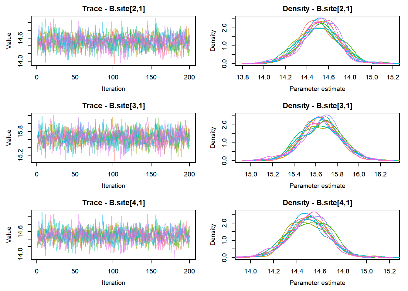
View traceplots ::: {.cell}
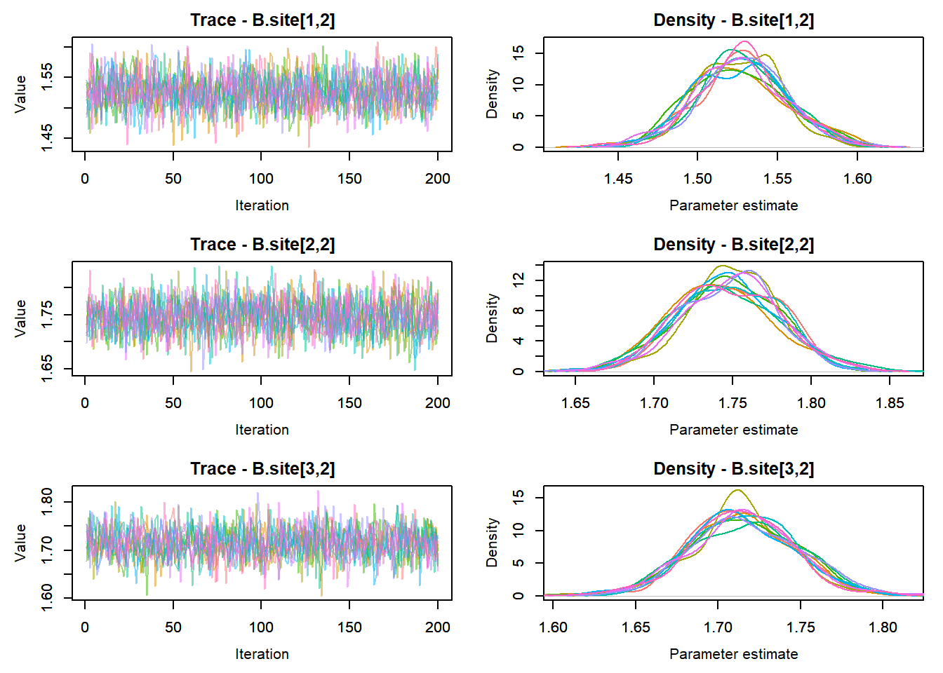
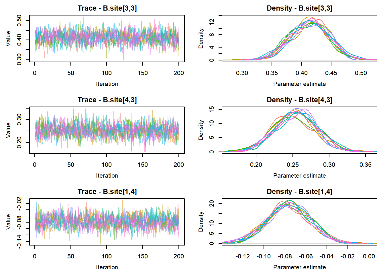
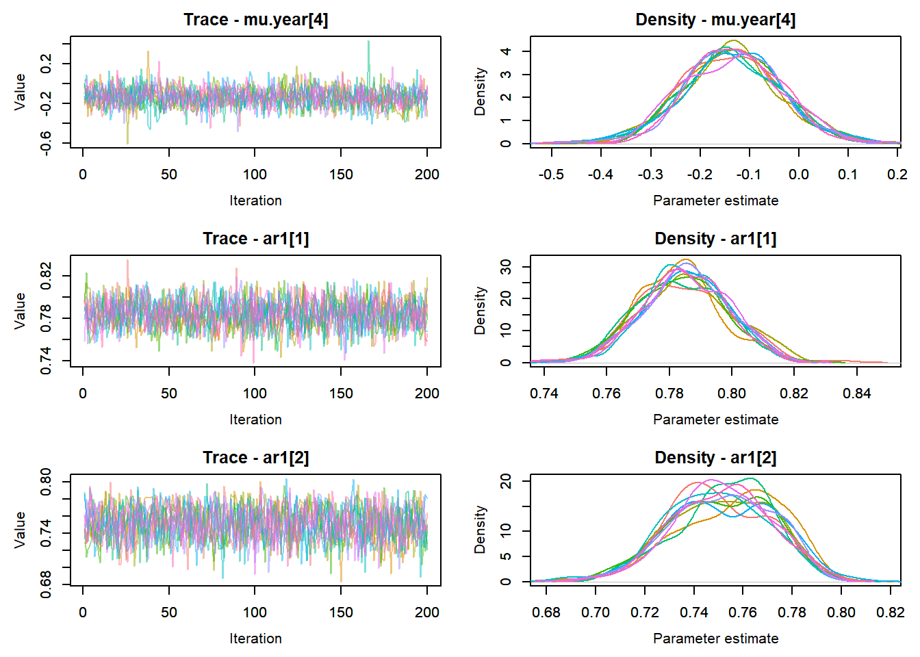
MCMCtrace(top_mod, ind = TRUE,
          params = c("B.0", "B.site", "mu.year",
                     "ar1",
                     "sigma"), pdf = FALSE)


:::
Convert to ggs object ::: {.cell}
ggfit <- ggs(as.mcmc(top_mod), keep_original_order = TRUE)
head(ggfit)
# A tibble: 6 × 4
Iteration Chain Parameter value
<int> <int> <fct> <dbl>
1 1 1 ar1[1] 0.794
2 2 1 ar1[1] 0.777
3 3 1 ar1[1] 0.784
4 4 1 ar1[1] 0.805
5 5 1 ar1[1] 0.789
6 6 1 ar1[1] 0.785:::
Format observed and predicted values ::: {.cell}
Mcmcdat <- as_tibble(Mcmcdat)

# subset expected and observed MCMC samples
ppdat_exp <- as.matrix(Mcmcdat[,startsWith(names(Mcmcdat), "stream.mu[")])
ppdat_obs <- as.matrix(Mcmcdat[,startsWith(names(Mcmcdat), "temp[")])
:::
Bayesian p-value ::: {.cell}
sum(ppdat_exp > ppdat_obs) / (dim(ppdat_obs)[1]*dim(ppdat_obs)[2])[1] 0.4987867:::
PP-check ::: {.cell}
ppdat_obs_mean <- apply(ppdat_obs, 2, mean)
ppdat_exp_mean <- apply(ppdat_exp, 2, mean)
tibble(obs = ppdat_obs_mean, exp = ppdat_exp_mean) %>%
  ggplot(aes(x = obs, y = exp)) +
  geom_point(alpha = 0.1) +
  # geom_smooth(method = "lm") +
  geom_abline(intercept = 0, slope = 1, color = "red") +
  theme_bw() + theme(panel.grid = element_blank()) +
  xlab("Observed") + ylab("Predicted (mean)")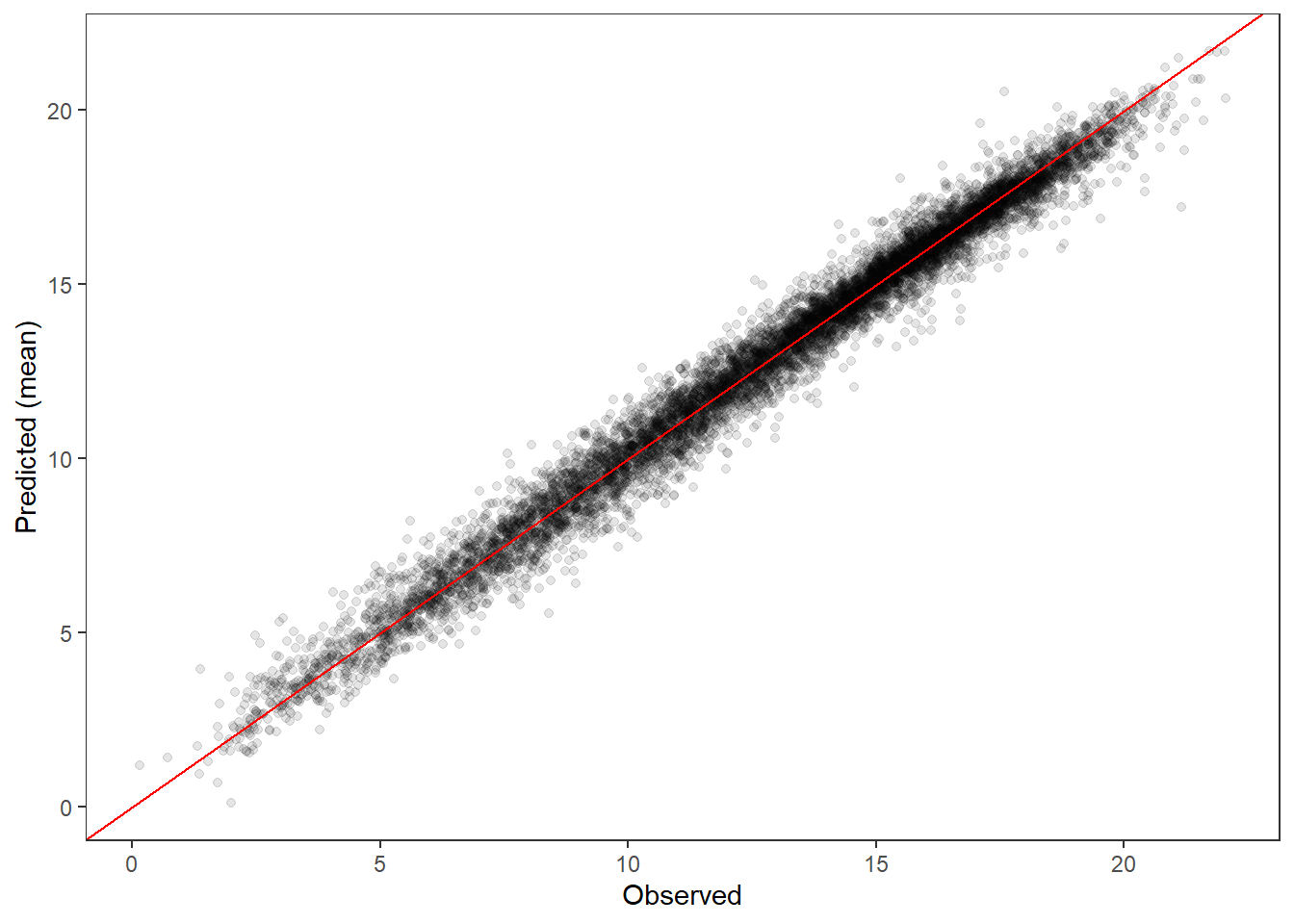
:::
Output is the same! Good!
Intercepts ::: {.cell}
ggfit %>%
  filter(Parameter %in% c("B.site[1,1]", "B.site[2,1]", "B.site[3,1]", "B.site[4,1]")) %>%
  mutate(Parameter = factor(Parameter, levels = c("B.site[1,1]", "B.site[2,1]", "B.site[3,1]", "B.site[4,1]"))) %>%
  ggs_caterpillar(sort = FALSE) +
  scale_y_discrete(labels = rev(c("int_WB", "int_OL", "int_OS", "int_IS")), limits = rev) +
  ylab("Intercepts") +
  theme_bw()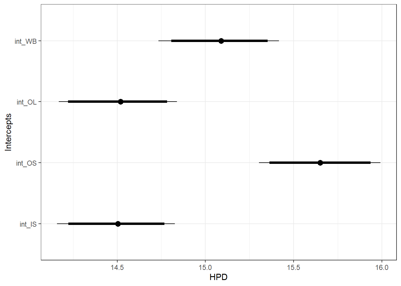
:::
Slopes, temperature effect ::: {.cell}
ggfit %>%
  filter(Iteration > 125) %>%
  filter(Parameter %in% c("B.site[1,2]", "B.site[2,2]", "B.site[3,2]", "B.site[4,2]")) %>%
  mutate(Parameter = factor(Parameter, levels = c("B.site[1,2]", "B.site[2,2]", "B.site[3,2]", "B.site[4,2]"))) %>%
  ggs_caterpillar(sort = FALSE) +
  scale_y_discrete(labels = rev(c("slo_WB", "slo_OL", "slo_OS", "slo_IS")), limits = rev) +
  ylab("Slopes, temperature effect") +
  theme_bw()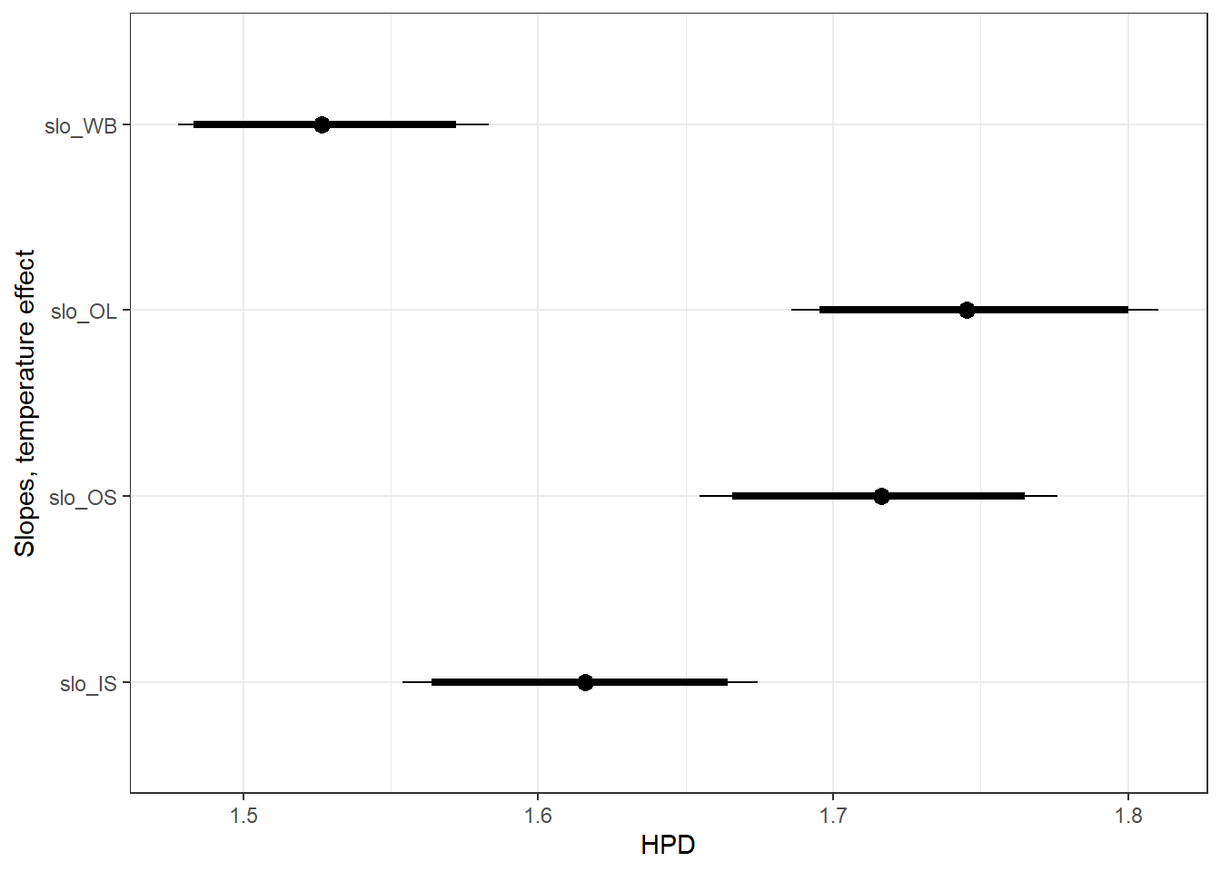
:::
Use the same hierarchical model as above, but allow effect of flow and flow-temp interaction to vary by site.
Get first observation indices and check that nFirstRowObs equals the number of unique site-years: must be TRUE! ::: {.cell}
# row indices for first observation in each site-year
firstObsRows <- unlist(tempDataSyncS %>%
  group_by(siteYear) %>%
  summarize(index = rowNum[min(which(!is.na(temp)))]) %>%
  ungroup() %>%
  select(index))
nFirstObsRows <- length(firstObsRows)

# does the number of first observations match the number of site years?
nFirstObsRows == length(unique(tempDataSyncS$siteYear))
[1] TRUE:::
Get row indices for all other observations ::: {.cell}
evalRows <- unlist(tempDataSyncS %>% filter(!rowNum %in% firstObsRows) %>% select(rowNum))
nEvalRows <- length(evalRows)
:::
Fixed and random effect data ::: {.cell}
data.random <- data.frame(intercept = 1,
                          airTemp = tempDataSyncS$airTemp,
                          flow =  tempDataSyncS$flowLS,
                          airFlow = tempDataSyncS$airTemp * tempDataSyncS$flowLS)

data.fixed <- data.frame(#intercept = 1
                         #,airTemp = tempDataSyncS$airTemp
                         airTempLag1 = tempDataSyncS$airTempLagged1
                         ,airTempLag2 = tempDataSyncS$airTempLagged2

                         # ,flow =  tempDataSyncS$flowLS
                         #
                         # ,airFlow = tempDataSyncS$airTemp * tempDataSyncS$flowLS
#                         ,air1Flow = tempDataSyncS$airTempLagged1 * tempDataSyncS$flowLS
#                         ,air2Flow = tempDataSyncS$airTempLagged2 * tempDataSyncS$flowLS

                         #main river effects
                         # ,river1 = tempDataSyncS$river1
                         # ,river2 = tempDataSyncS$river2
                         # ,river3 = tempDataSyncS$river3
                         #
                         # #river interaction with air temp
                         # ,river1Air = tempDataSyncS$river1 * tempDataSyncS$airTemp
                         # ,river2Air = tempDataSyncS$river2 * tempDataSyncS$airTemp
                         # ,river3Air = tempDataSyncS$river3 * tempDataSyncS$airTemp

                          )

data.random.years <- data.frame(intercept.year = 1,
                     dOY  = tempDataSyncS$dOY,
                     dOY2 = tempDataSyncS$dOY^2,
                     dOY3 = tempDataSyncS$dOY^3
                     )
:::
Misc. objects ::: {.cell}
Ti <- length(unique(tempDataSyncS$year))
L <- dim(data.random.years)[2]
W.year <- diag(L)
:::
Combine data in list ::: {.cell}
# combine data in a list
jags.data <- list("temp" = tempDataSyncS$temp,
                  "nFirstObsRows" = nFirstObsRows,
                  "firstObsRows" = firstObsRows,
                  "nEvalRows" = nEvalRows,
                  "evalRows" = evalRows,
                  "X.0" = as.matrix(data.fixed),
                  "X.site" = as.matrix(data.random),
                  "X.year" = as.matrix(data.random.years),
                  "Kfixed" = dim(data.fixed)[2],
                  "Krandom" = dim(data.random)[2],
                  "nsites" = length(unique(tempDataSyncS$site)),
                  "Ti" = Ti,
                  "L" = L,
                  "W.year" = W.year,
                  "n" = dim(tempDataSyncS)[1],
                  "year" = as.factor(tempDataSyncS$year),
                  "site" = as.numeric(tempDataSyncS$riverOrdered)
                  )
:::
Parameters to monitor ::: {.cell}
jags.params <- c("residuals",
            "deviance",
            #"pD",
            "sigma",
            "B.0",
            "B.site",
            "B.year",
            #"mu.B.river",
            "rho.B.year",
            "mu.year",
            "sigma.b.year",
            "stream.mu",
            "ar1" ,
            "ar1Mean",
            "ar1SD",
            "temp",
            "sigma.B.site"
            )
:::
fit0_h2 <- jags.parallel(data = jags.data, inits = NULL, parameters.to.save = jags.params,
                         model.file = "JAGS models/DailyTempModelJAGS_Letcher_hierarchical.txt",
                         n.chains = 10, n.thin = 10, n.burnin = 1000, n.iter = 3000, DIC = TRUE)
beep()Save to file ::: {.cell}
saveRDS(fit0_h2, "Model objects/LetcherTempModel_PeerJ2016_hierarchical.RDS"):::
Read in fitted model object ::: {.cell}
fit0_h2 <- readRDS("Model objects/LetcherTempModel_PeerJ2016_hierarchical.RDS"):::
Get MCMC samples and summary ::: {.cell}
top_mod <- fit0_h2
# generate MCMC samples and store as an array
modelout <- top_mod$BUGSoutput
McmcList <- vector("list", length = dim(modelout$sims.array)[2])
for(i in 1:length(McmcList)) { McmcList[[i]] = as.mcmc(modelout$sims.array[,i,]) }
# rbind MCMC samples from 10 chains
Mcmcdat <- rbind(McmcList[[1]], McmcList[[2]], McmcList[[3]], McmcList[[4]], McmcList[[5]], McmcList[[6]], McmcList[[7]], McmcList[[8]], McmcList[[9]], McmcList[[10]])
param.summary <- modelout$summary
head(param.summary)
mean sd 2.5% 25% 50% 75%
B.0[1] 0.1996561 0.01588663 0.1684552 0.1886198 0.1996409 0.2104592
B.0[2] 0.1601317 0.01647412 0.1274510 0.1493978 0.1605079 0.1708984
B.site[1,1] 15.0877438 0.17053466 14.7339107 14.9767446 15.0888867 15.2033860
B.site[2,1] 14.5154004 0.17175886 14.1691837 14.4035158 14.5196452 14.6311073
B.site[3,1] 15.6480333 0.17548672 15.3041803 15.5293132 15.6508855 15.7645190
B.site[4,1] 14.5004781 0.16993161 14.1586293 14.3871769 14.5034804 14.6162630
97.5% Rhat n.eff
B.0[1] 0.2306411 1.001439 1900
B.0[2] 0.1926820 1.002371 1400
B.site[1,1] 15.4179276 1.000438 2000
B.site[2,1] 14.8386405 1.001710 1700
B.site[3,1] 15.9918072 1.000590 2000
B.site[4,1] 14.8276109 1.001154 2000:::
Any problematic R-hat values (>1.05)? ::: {.cell}
top_mod$BUGSoutput$summary[,8][top_mod$BUGSoutput$summary[,8] > 1.05]residuals[7152]
1.056715 :::
View traceplots ::: {.cell}
MCMCtrace(top_mod, ind = TRUE,
          params = c("B.0", "B.site", "mu.year",
                     "ar1",
                     "sigma"), pdf = FALSE)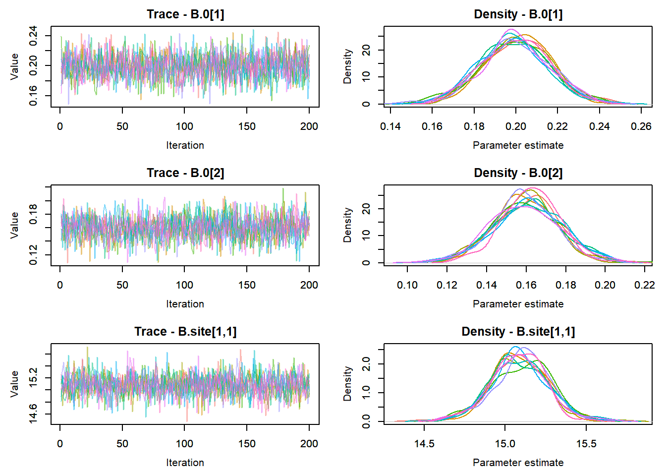

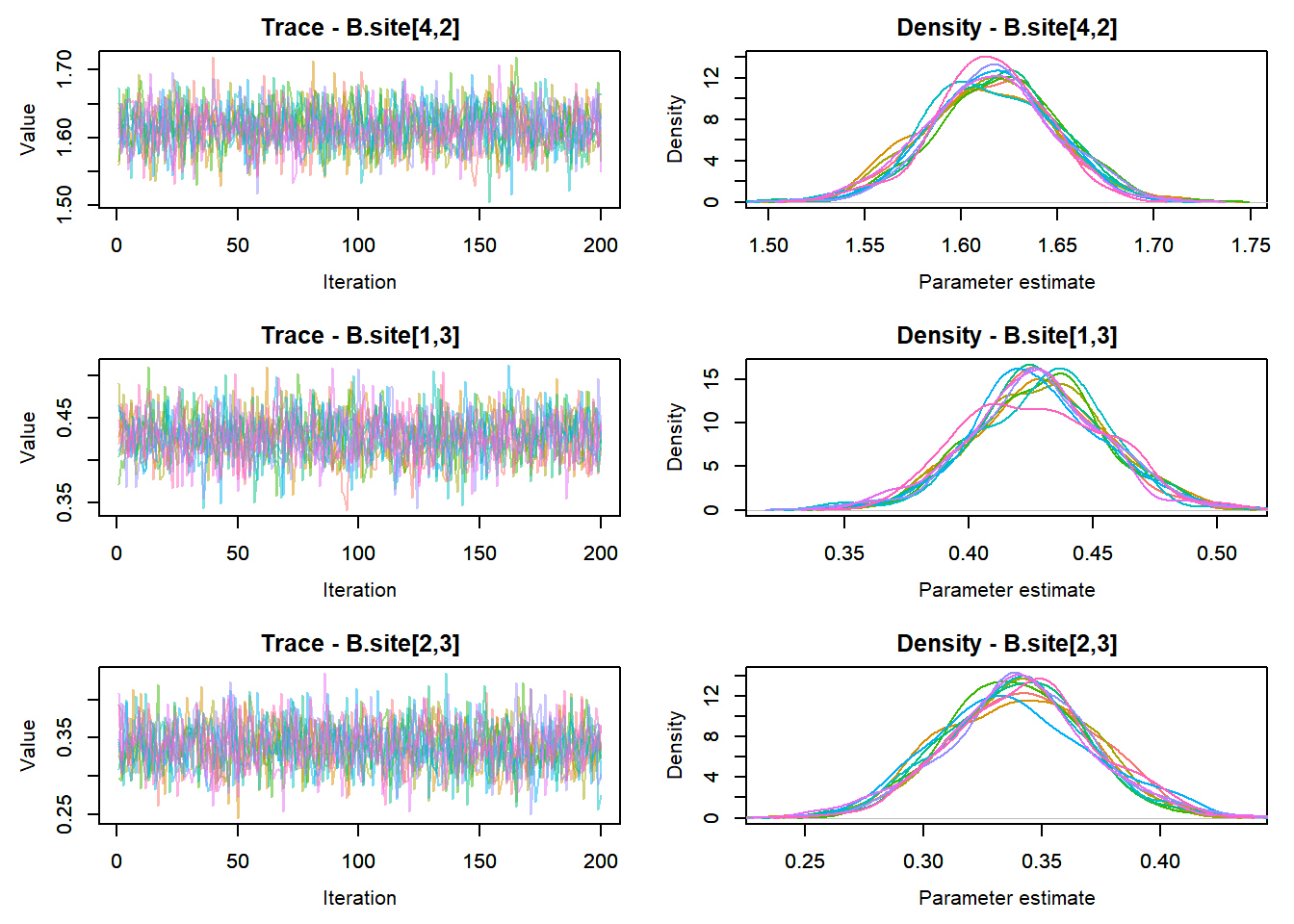

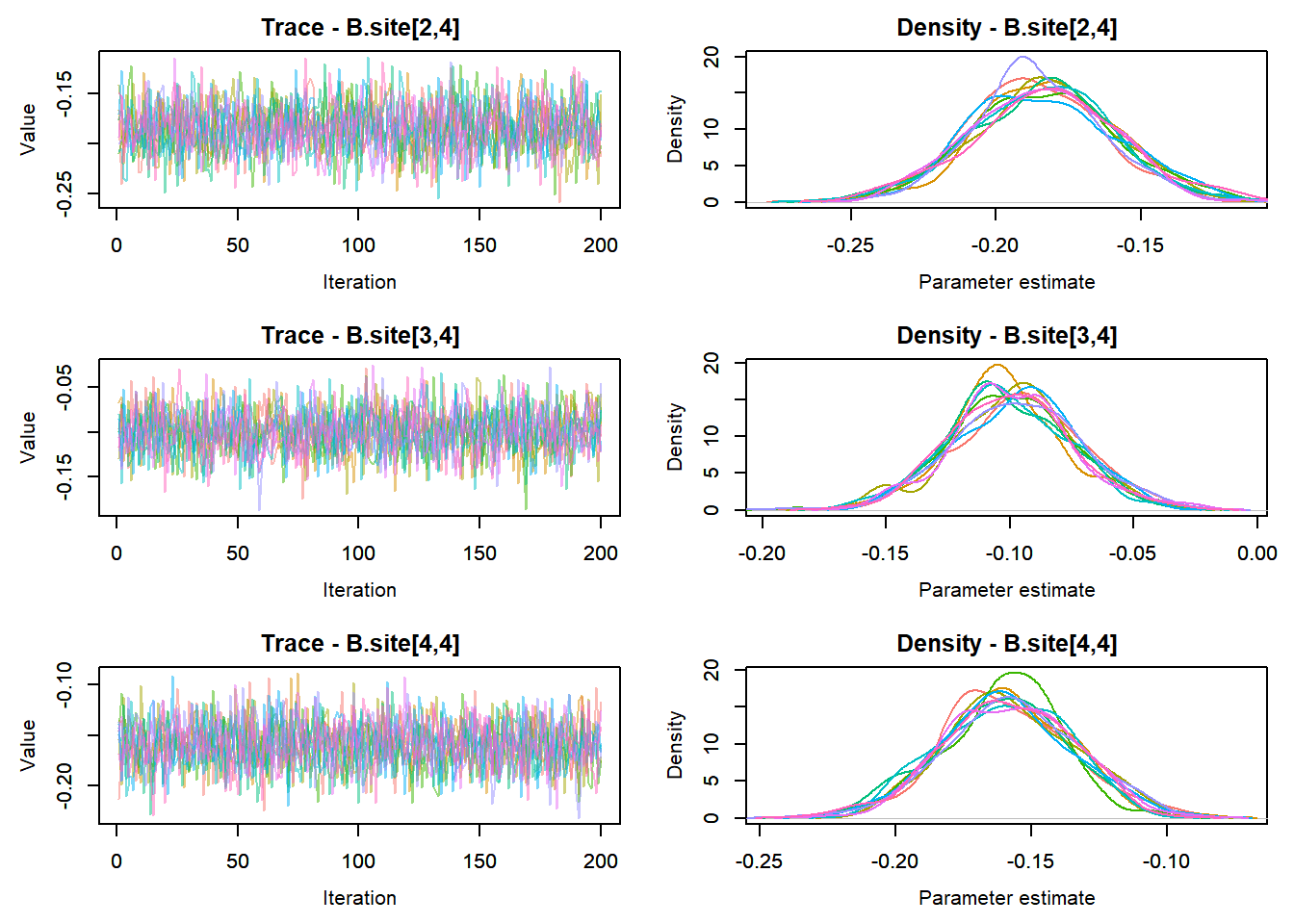
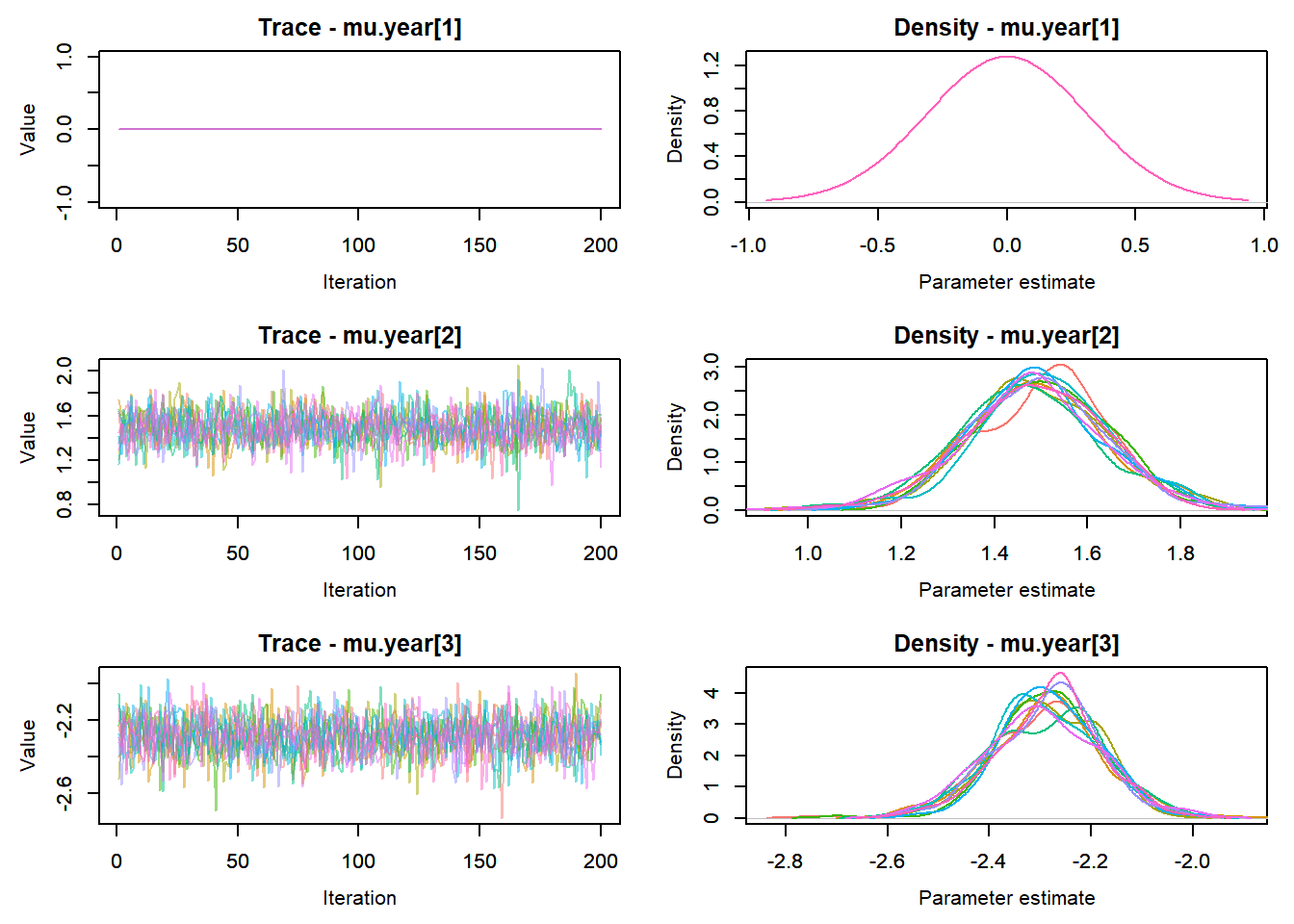

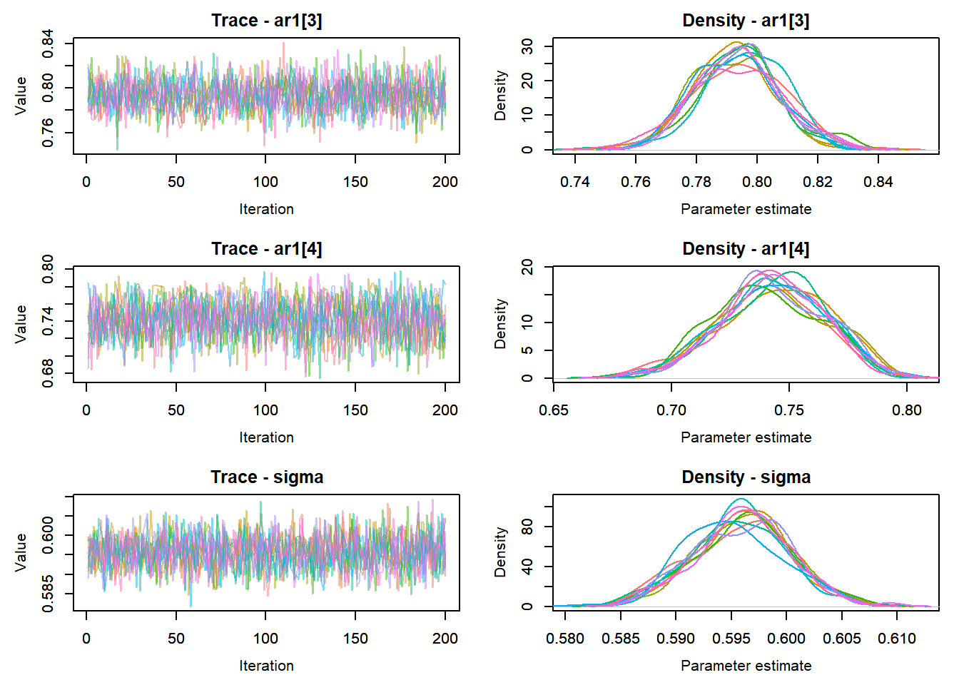
:::
Convert to ggs object ::: {.cell}
ggfit <- ggs(as.mcmc(top_mod), keep_original_order = TRUE)
head(ggfit)
# A tibble: 6 × 4
Iteration Chain Parameter value
<int> <int> <fct> <dbl>
1 1 1 ar1[1] 0.794
2 2 1 ar1[1] 0.777
3 3 1 ar1[1] 0.784
4 4 1 ar1[1] 0.805
5 5 1 ar1[1] 0.789
6 6 1 ar1[1] 0.785:::
Format observed and predicted values ::: {.cell}
Mcmcdat <- as_tibble(Mcmcdat)

# subset expected and observed MCMC samples
ppdat_exp <- as.matrix(Mcmcdat[,startsWith(names(Mcmcdat), "stream.mu[")])
ppdat_obs <- as.matrix(Mcmcdat[,startsWith(names(Mcmcdat), "temp[")])
:::
Bayesian p-value ::: {.cell}
sum(ppdat_exp > ppdat_obs) / (dim(ppdat_obs)[1]*dim(ppdat_obs)[2])[1] 0.4987867:::
PP-check ::: {.cell}
ppdat_obs_mean <- apply(ppdat_obs, 2, mean)
ppdat_exp_mean <- apply(ppdat_exp, 2, mean)
tibble(obs = ppdat_obs_mean, exp = ppdat_exp_mean) %>%
  ggplot(aes(x = obs, y = exp)) +
  geom_point(alpha = 0.1) +
  # geom_smooth(method = "lm") +
  geom_abline(intercept = 0, slope = 1, color = "red") +
  theme_bw() + theme(panel.grid = element_blank()) +
  xlab("Observed") + ylab("Predicted (mean)")
:::
ggfit %>%
  filter(Parameter %in% c("B.site[1,1]", "B.site[2,1]", "B.site[3,1]", "B.site[4,1]")) %>%
  mutate(Parameter = factor(Parameter, levels = c("B.site[1,1]", "B.site[2,1]", "B.site[3,1]", "B.site[4,1]"))) %>%
  ggs_caterpillar(sort = FALSE) +
  scale_y_discrete(labels = rev(c("int_WB", "int_OL", "int_OS", "int_IS")), limits = rev) +
  ylab("Intercepts") +
  theme_bw()
ggfit %>%
  filter(Parameter %in% c("B.site[1,2]", "B.site[2,2]", "B.site[3,2]", "B.site[4,2]")) %>%
  mutate(Parameter = factor(Parameter, levels = c("B.site[1,2]", "B.site[2,2]", "B.site[3,2]", "B.site[4,2]"))) %>%
  ggs_caterpillar(sort = FALSE) +
  scale_y_discrete(labels = rev(c("slo_WB", "slo_OL", "slo_OS", "slo_IS")), limits = rev) +
  ylab("Slopes, temperature effect") +
  theme_bw()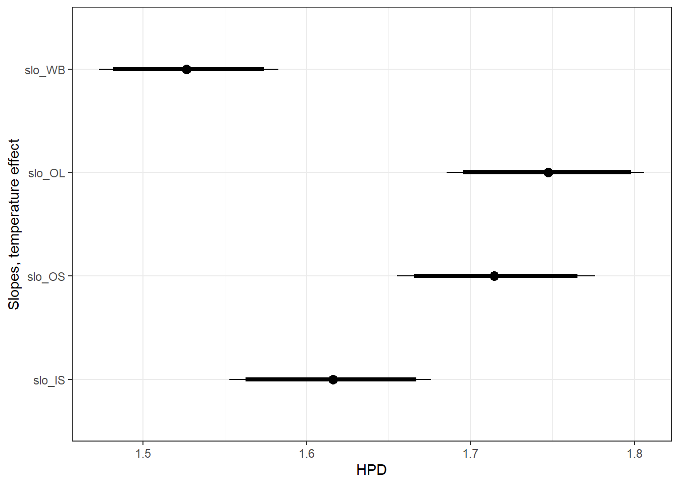
ggfit %>%
  filter(Parameter %in% c("B.site[1,3]", "B.site[2,3]", "B.site[3,3]", "B.site[4,3]")) %>%
  mutate(Parameter = factor(Parameter, levels = c("B.site[1,3]", "B.site[2,3]", "B.site[3,3]", "B.site[4,3]"))) %>%
  ggs_caterpillar(sort = FALSE) +
  scale_y_discrete(labels = rev(c("slo_WB", "slo_OL", "slo_OS", "slo_IS")), limits = rev) +
  ylab("Slopes, flow effect") +
  theme_bw()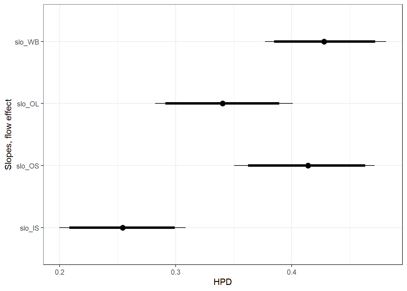
ggfit %>%
  filter(Parameter %in% c("B.site[1,4]", "B.site[2,4]", "B.site[3,4]", "B.site[4,4]")) %>%
  mutate(Parameter = factor(Parameter, levels = c("B.site[1,4]", "B.site[2,4]", "B.site[3,4]", "B.site[4,4]"))) %>%
  ggs_caterpillar(sort = FALSE) +
  scale_y_discrete(labels = rev(c("slo_WB", "slo_OL", "slo_OS", "slo_IS")), limits = rev) +
  ylab("Slopes, temp-flow interaction") +
  theme_bw()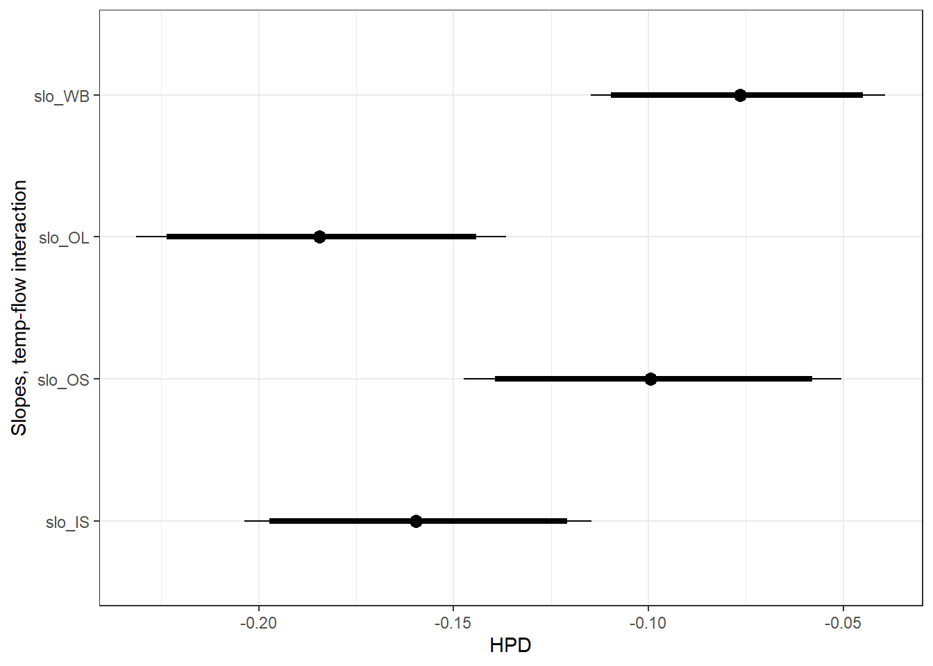
ggs_caterpillar(ggfit %>% filter(Parameter %in% grep("ar1", unique(ggfit$Parameter), value = TRUE)) %>%
                  mutate(Parameter = factor(Parameter, levels = c("ar1Mean", "ar1SD", "ar1[1]", "ar1[2]", "ar1[3]", "ar1[4]"))),
                sort = FALSE) + scale_y_discrete(labels = rev(c("ar1Mean", "ar1SD", "ar1[WB]", "ar1[OL]", "ar1[OS]", "ar1[IL]")), limits = rev) + theme_bw() + xlim(0,1)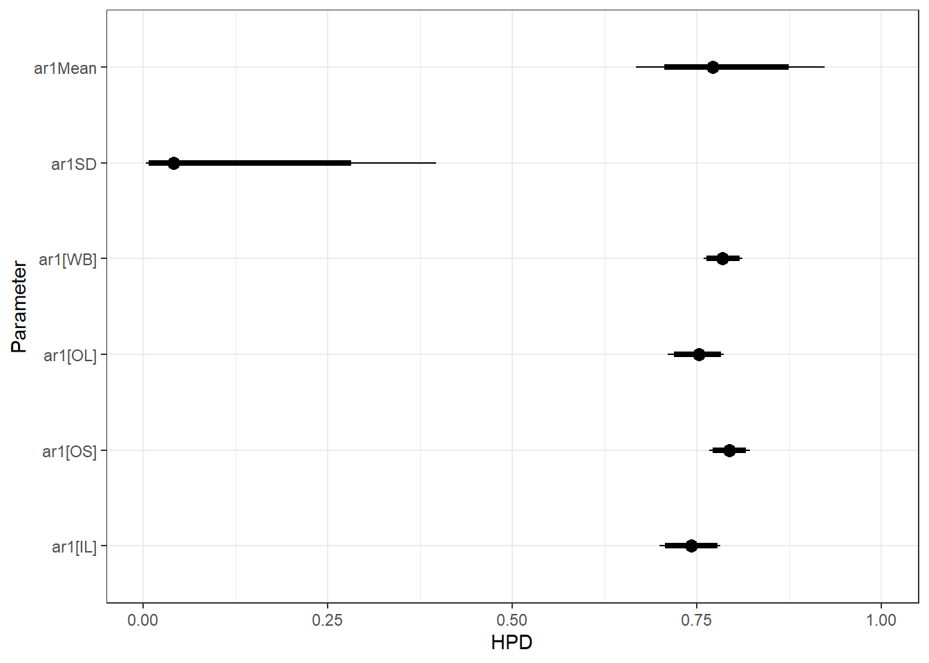
ggs_caterpillar(ggfit, family = "mu.year", sort = FALSE) + scale_y_discrete(labels = rev(c("Intercept", "Linear", "Quadratic", "Cubic")), limits = rev) + theme_bw()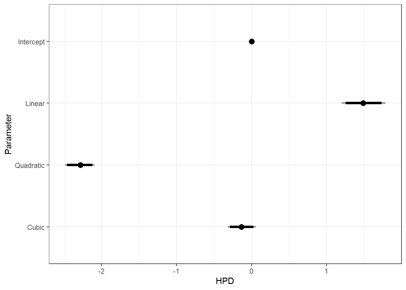
Marginal effects of air temperature x flow interaction, not accounting for lagged temperature effects, temporal autocorrelation,
# set up
np <- 100
myriv <- "WEST BROOK"
x_temp <- seq(from = min(tempDataSyncS$airTemp[tempDataSyncS$riverOrdered == myriv]),
              to = max(tempDataSyncS$airTemp[tempDataSyncS$riverOrdered == myriv]),
              length.out = np)
x_flow <- seq(from = min(tempDataSyncS$flowLS[tempDataSyncS$riverOrdered == myriv]),
              to = max(tempDataSyncS$flowLS[tempDataSyncS$riverOrdered == myriv]),
              length.out = np)
pred_df <- expand_grid(x_temp, x_flow)

# predict from model
pred_df$pred <- param.summary["B.site[1,1]",1] + param.summary["B.site[1,2]",1]*pred_df$x_temp + param.summary["B.site[1,3]",1]*pred_df$x_flow + param.summary["B.site[1,4]",1]*pred_df$x_temp*pred_df$x_flow

# lines
p1 <- ggplot(pred_df, aes(x = x_temp, y = pred, color = x_flow, group = x_flow)) +
  geom_line() +
  scale_color_distiller(palette = "BrBG", direction = +1) +
  theme_bw() + theme(panel.grid = element_blank()) +
  labs(color = "Flow") + xlab("Air temperature") + ylab("Water temperature") + ylim(6.5,20)
# heatmap
p2 <- ggplot(pred_df, aes(x = x_temp, y = x_flow)) +
  geom_tile(aes(fill = pred)) +
  scale_fill_distiller(palette = "Spectral", limits = c(6.5,20)) +
  theme_bw() + theme(panel.grid = element_blank()) +
  scale_x_continuous(expand = c(0,0)) + scale_y_continuous(expand = c(0,0)) +
  labs(fill = "Water\ntemp.") + xlab("Air temperature") + ylab("Flow") #+
  #geom_point(data = tempDataSyncS %>% filter(riverOrdered == myriv), aes(x = airTemp, y = flowLS, color = temp)) +
  #scale_color_distiller(palette = "Spectral", limits = c(0,23))
# combine
egg::ggarrange(p1, p2, nrow = 1)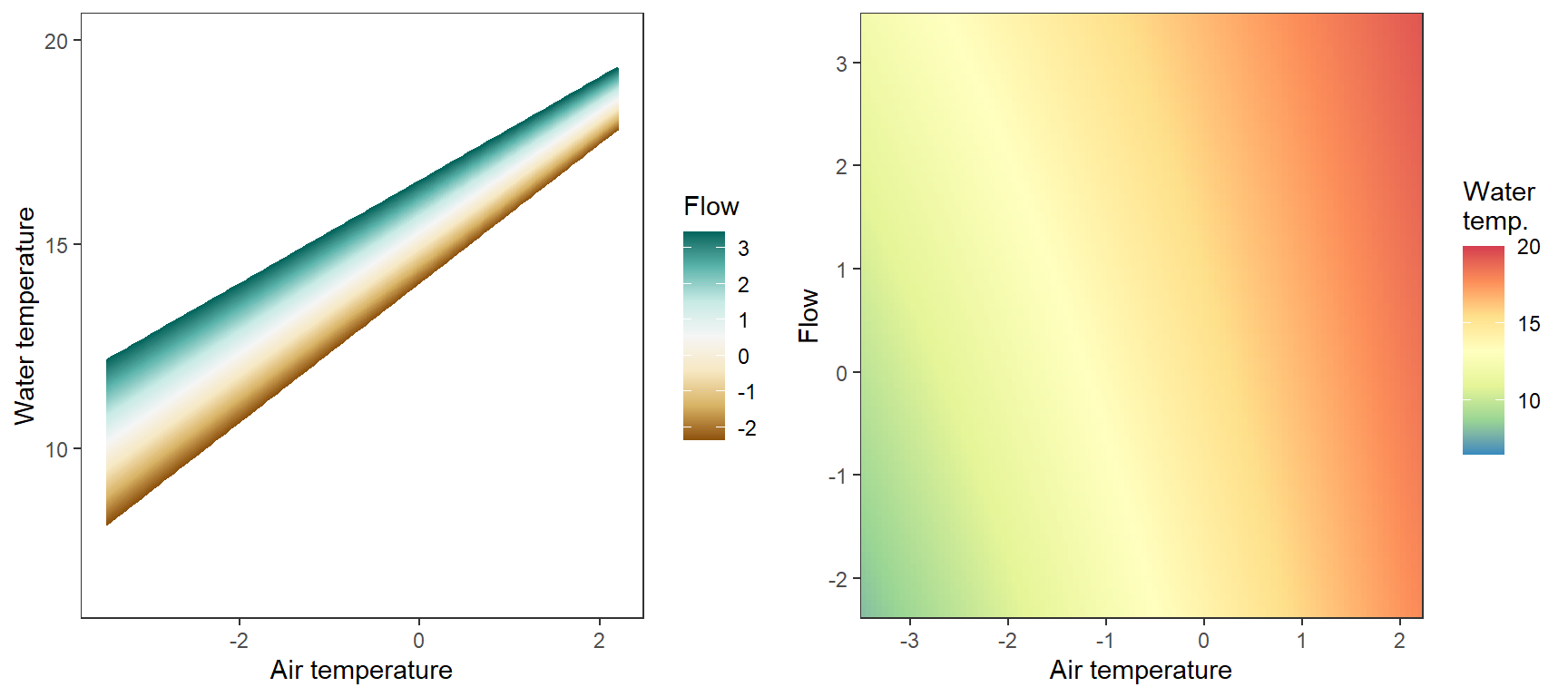
# set up
np <- 100
myriv <- "WB JIMMY"
x_temp <- seq(from = min(tempDataSyncS$airTemp[tempDataSyncS$riverOrdered == myriv]),
              to = max(tempDataSyncS$airTemp[tempDataSyncS$riverOrdered == myriv]),
              length.out = np)
x_flow <- seq(from = min(tempDataSyncS$airTemp[tempDataSyncS$riverOrdered == myriv]),
              to = max(tempDataSyncS$airTemp[tempDataSyncS$riverOrdered == myriv]),
              length.out = np)
pred_df <- expand_grid(x_temp, x_flow)

# predict from model
pred_df$pred <- param.summary["B.site[2,1]",1] + param.summary["B.site[2,2]",1]*pred_df$x_temp + param.summary["B.site[2,3]",1]*pred_df$x_flow + param.summary["B.site[2,4]",1]*pred_df$x_temp*pred_df$x_flow

# lines
p1 <- ggplot(pred_df, aes(x = x_temp, y = pred, color = x_flow, group = x_flow)) +
  geom_line() +
  scale_color_distiller(palette = "BrBG", direction = +1) +
  theme_bw() + theme(panel.grid = element_blank()) +
  labs(color = "Flow") + xlab("Air temperature") + ylab("Water temperature") + ylim(6.5,20)
# heatmap
p2 <- ggplot(pred_df, aes(x = x_temp, y = x_flow)) +
  geom_tile(aes(fill = pred)) +
  scale_fill_distiller(palette = "Spectral", limits = c(6.5,20)) +
  theme_bw() + theme(panel.grid = element_blank()) +
  scale_x_continuous(expand = c(0,0)) + scale_y_continuous(expand = c(0,0)) +
  labs(fill = "Water\ntemp.") + xlab("Air temperature") + ylab("Flow")
# combine
egg::ggarrange(p1, p2, nrow = 1)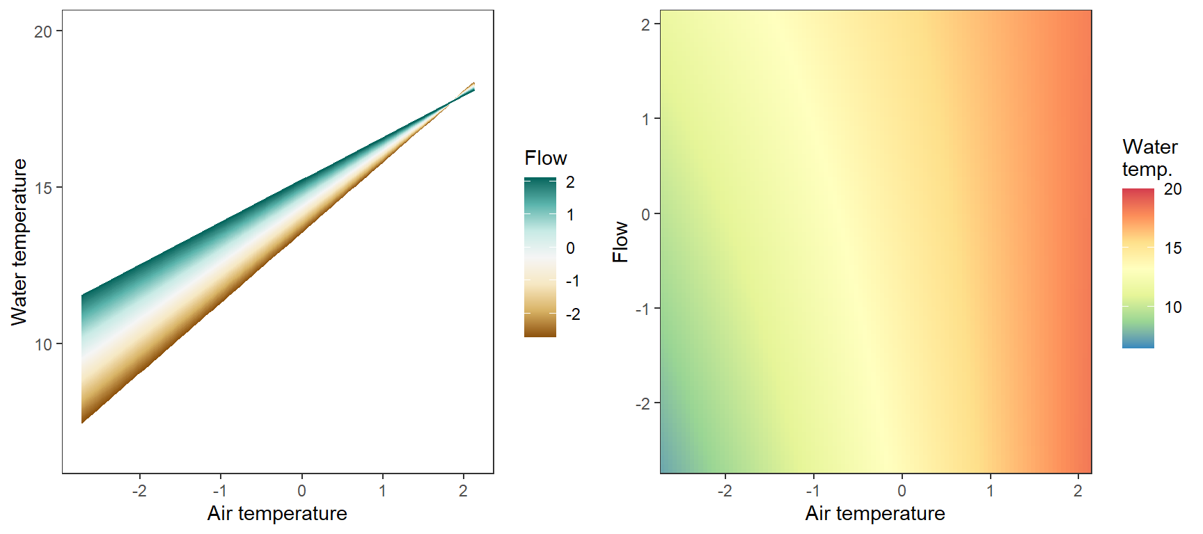
# set up
np <- 100
myriv <- "WB MITCHELL"
x_temp <- seq(from = min(tempDataSyncS$airTemp[tempDataSyncS$riverOrdered == myriv]),
              to = max(tempDataSyncS$airTemp[tempDataSyncS$riverOrdered == myriv]),
              length.out = np)
x_flow <- seq(from = min(tempDataSyncS$airTemp[tempDataSyncS$riverOrdered == myriv]),
              to = max(tempDataSyncS$airTemp[tempDataSyncS$riverOrdered == myriv]),
              length.out = np)
pred_df <- expand_grid(x_temp, x_flow)

# predict from model
pred_df$pred <- param.summary["B.site[3,1]",1] + param.summary["B.site[3,2]",1]*pred_df$x_temp + param.summary["B.site[3,3]",1]*pred_df$x_flow + param.summary["B.site[3,4]",1]*pred_df$x_temp*pred_df$x_flow

# lines
p1 <- ggplot(pred_df, aes(x = x_temp, y = pred, color = x_flow, group = x_flow)) +
  geom_line() +
  scale_color_distiller(palette = "BrBG", direction = +1) +
  theme_bw() + theme(panel.grid = element_blank()) +
  labs(color = "Flow") + xlab("Air temperature") + ylab("Water temperature") + ylim(6.5,20)
# heatmap
p2 <- ggplot(pred_df, aes(x = x_temp, y = x_flow)) +
  geom_tile(aes(fill = pred)) +
  scale_fill_distiller(palette = "Spectral", limits = c(6.5,20)) +
  theme_bw() + theme(panel.grid = element_blank()) +
  scale_x_continuous(expand = c(0,0)) + scale_y_continuous(expand = c(0,0)) +
  labs(fill = "Water\ntemp.") + xlab("Air temperature") + ylab("Flow")
# combine
egg::ggarrange(p1, p2, nrow = 1)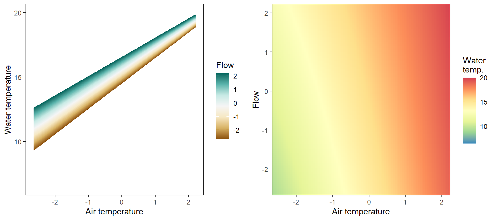
# set up
np <- 100
myriv <- "WB OBEAR"
x_temp <- seq(from = min(tempDataSyncS$airTemp[tempDataSyncS$riverOrdered == myriv]),
              to = max(tempDataSyncS$airTemp[tempDataSyncS$riverOrdered == myriv]),
              length.out = np)
x_flow <- seq(from = min(tempDataSyncS$airTemp[tempDataSyncS$riverOrdered == myriv]),
              to = max(tempDataSyncS$airTemp[tempDataSyncS$riverOrdered == myriv]),
              length.out = np)
pred_df <- expand_grid(x_temp, x_flow)

# predict from model
pred_df$pred <- param.summary["B.site[4,1]",1] + param.summary["B.site[4,2]",1]*pred_df$x_temp + param.summary["B.site[4,3]",1]*pred_df$x_flow + param.summary["B.site[4,4]",1]*pred_df$x_temp*pred_df$x_flow

# lines
p1 <- ggplot(pred_df, aes(x = x_temp, y = pred, color = x_flow, group = x_flow)) +
  geom_line() +
  scale_color_distiller(palette = "BrBG", direction = +1) +
  theme_bw() + theme(panel.grid = element_blank()) +
  labs(color = "Flow") + xlab("Air temperature") + ylab("Water temperature") + ylim(6.5,20)
# heatmap
p2 <- ggplot(pred_df, aes(x = x_temp, y = x_flow)) +
  geom_tile(aes(fill = pred)) +
  scale_fill_distiller(palette = "Spectral", limits = c(6.5,20)) +
  theme_bw() + theme(panel.grid = element_blank()) +
  scale_x_continuous(expand = c(0,0)) + scale_y_continuous(expand = c(0,0)) +
  labs(fill = "Water\ntemp.") + xlab("Air temperature") + ylab("Flow")
# combine
egg::ggarrange(p1, p2, nrow = 1)