6 GCM Data Summary

Purpose: Generate future seasonal mean air temperature projections from GCM data (Rahimi et al. 2024, Geoscientific Model Development)

6.1 Generate seasonal projections

Some misc. objects

Code

patt <- c("t2min_atStation_corrected", "t2max_atStation_corrected", "t2min_atStation_original", "t2max_atStation_original")
summ <- c("min", "max", "min", "max")
type <- c("corrected", "corrected", "original", "original")
mylist <- list()

Pull in climate projection data

Code

for(i in 1:length(patt)) {
  myfiles <- list.files("Data/GCM Archive", pattern = patt[i], full.names = TRUE)
  dat <- read_csv(myfiles, id = "file_name")[,c(1,2,5)] %>% mutate(summ = summ[i], type = type[i], gcm = str_match(file_name, "Archive/\\s*(.*?)\\s*_t2")[,2])
  dat <- dat %>% select(6,4,5,2,3) %>% rename(date = 4, temp = 5)
  mylist[[i]] <- dat
  #print(i)
}
dat <- do.call(rbind, mylist)
summary(dat)

     gcm                summ               type                date           
 Length:2604648     Length:2604648     Length:2604648     Min.   :1980-10-01  
 Class :character   Class :character   Class :character   1st Qu.:2010-07-01  
 Mode  :character   Mode  :character   Mode  :character   Median :2040-04-01  
                                                          Mean   :2040-03-31  
                                                          3rd Qu.:2069-12-31  
                                                          Max.   :2099-09-30  
                                                          NA's   :836         
      temp      
 Min.   :217.5  
 1st Qu.:269.5  
 Median :276.6  
 Mean   :277.9  
 3rd Qu.:286.6  
 Max.   :315.6

Code

head(dat)

# A tibble: 6 × 5
  gcm                 summ  type      date        temp
  <chr>               <chr> <chr>     <date>     <dbl>
1 access-cm2_r5i1p1f1 min   corrected 1980-10-01  268.
2 access-cm2_r5i1p1f1 min   corrected 1980-10-02  257.
3 access-cm2_r5i1p1f1 min   corrected 1980-10-03  253.
4 access-cm2_r5i1p1f1 min   corrected 1980-10-04  260.
5 access-cm2_r5i1p1f1 min   corrected 1980-10-05  267.
6 access-cm2_r5i1p1f1 min   corrected 1980-10-06  271.

Notes:

Some GCMs do not predict for Feb 29 (leap years)
ukesm1-0-ll_r2i1p1f2 predicts for 30 days per month, even in Feb (but does not actually have dates for Feb 29/30)

Code

view(dat %>% group_by(gcm, summ, type) %>% summarise(mind = min(date, na.rm = T), maxd = max(date, na.rm = T), n = n()))

Some GCMs do not predict for Feb 29 (leap years)…drop NAs

Code

dat <- dat %>% filter(!is.na(date))

Find daily mean temp for each climate model

Code

dat2 <- dat %>% group_by(gcm, type, date) %>% summarize(temp_mean = mean(temp)-273.15) %>% ungroup()
dat2 %>% group_by(gcm) %>% summarise(mind = min(date), maxd = max(date), n = n())

# A tibble: 15 × 4
   gcm                    mind       maxd           n
   <chr>                  <date>     <date>     <int>
 1 access-cm2_r5i1p1f1    1980-10-01 2099-09-30 86928
 2 canesm5_r1i1p2f1       1980-10-01 2099-09-30 86870
 3 cesm2_r11i1p1f1        1980-10-01 2099-09-30 86870
 4 cnrm-esm2-1_r1i1p1f2   1980-10-01 2099-09-30 86928
 5 ec-earth3-veg_r1i1p1f1 1980-10-01 2099-09-30 86928
 6 ec-earth3_r1i1p1f1     1980-10-01 2099-09-30 86928
 7 fgoals-g3_r1i1p1f1     1980-10-01 2099-09-30 86870
 8 giss-e2-1-g_r1i1p1f2   1980-10-01 2099-09-30 86870
 9 miroc6_r1i1p1f1        1980-10-01 2099-09-30 86928
10 mpi-esm1-2-hr_r3i1p1f1 1980-10-01 2099-09-30 86928
11 mpi-esm1-2-hr_r7i1p1f1 1980-10-01 2099-09-30 86928
12 mpi-esm1-2-lr_r7i1p1f1 1980-10-01 2099-09-30 86928
13 noresm2-mm_r1i1p1f1    1980-10-01 2099-09-30 86870
14 taiesm1_r1i1p1f1       1980-10-01 2099-09-30 86870
15 ukesm1-0-ll_r2i1p1f2   1980-10-01 2099-09-30 85262

Code

#sum(is.na(dat2$temp_mean))

6.1.1 Vizualize raw GCM data

Group by year, plot time series of annual means.

Code

dat2 %>% mutate(year = year(date)) %>% group_by(gcm, year) %>% summarize(ann_temp = mean(temp_mean)) %>% ggplot() + geom_line(aes(x = year, y = ann_temp, group = gcm, colour = gcm))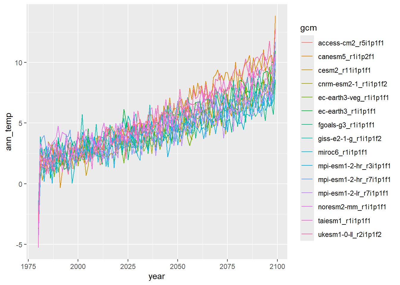

View corrected daily (mean) air temp for a single year (1981)

Code

dat2 %>% filter(date >= "1981-01-01" & date <= "1981-12-31", type == "corrected") %>% ggplot() + geom_line(aes(x = date, y = temp_mean, group = gcm, colour = gcm))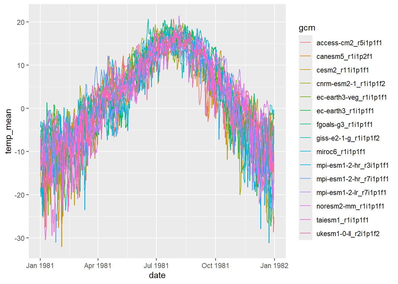

6.1.2 Summarize across seasons

Summarize GCM data across four seasons

Code

dat2 <- dat2 %>% mutate(season = ifelse(month(date) %in% c(9,10,11), "fal",
                                        ifelse(month(date) %in% c(12,1,2), "win",
                                               ifelse(month(date) %in% c(3,4,5), "spr", "sum"))))
dat3 <- dat2 %>% group_by(gcm, type, season, year(date)) %>% summarize(temp_mean = mean(temp_mean)) %>% rename(year = 4)

Plot time series of seasonal mean air temperature:

Code

dat3 %>% ggplot() + geom_line(aes(x = year, y = temp_mean, group = gcm, colour = gcm)) + facet_wrap(~season)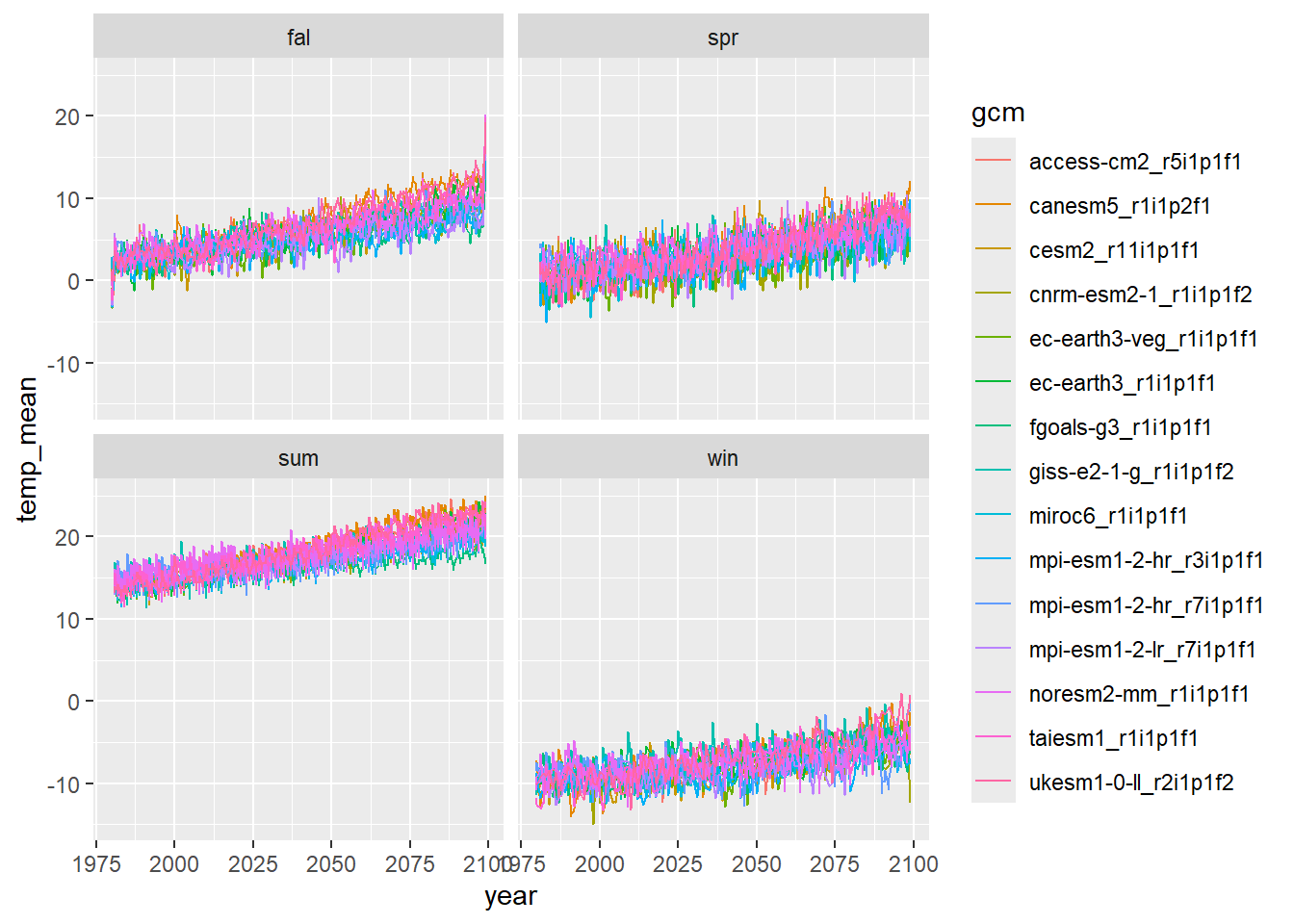

6.1.3 Summarize across GCMs

Summarize seasonal mean air temperature across 15 GCMs

Code

dat_summ <- dat3 %>% group_by(type, season, year) %>% summarize(count = n(), temp_avg = mean(temp_mean, na.rm = T), temp_sd = sd(temp_mean, na.rm = T), temp_min = min(temp_mean, na.rm = T), temp_max = max(temp_mean, na.rm = T)) %>% ungroup()

Plot raw and corrected output: mean min and max

Code

dat_summ %>% ggplot() + geom_line(aes(x = year, y = temp_avg)) + geom_line(aes(x = year, y = temp_min), color = 4) + geom_line(aes(x = year, y = temp_max), color = 2) + facet_wrap(~season + type)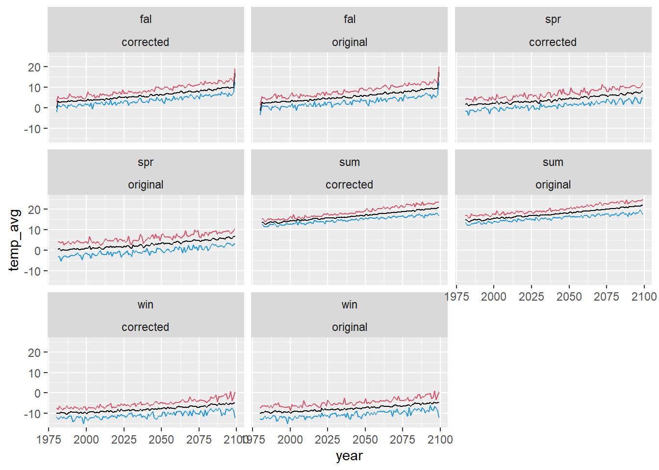

View winter corrected only:

Code

dat_summ %>% filter(season == "win", type == "corrected") %>% ggplot() + geom_line(aes(x = year, y = temp_avg)) + geom_line(aes(x = year, y = temp_min), linetype = 2) + geom_line(aes(x = year, y = temp_max), linetype = 2)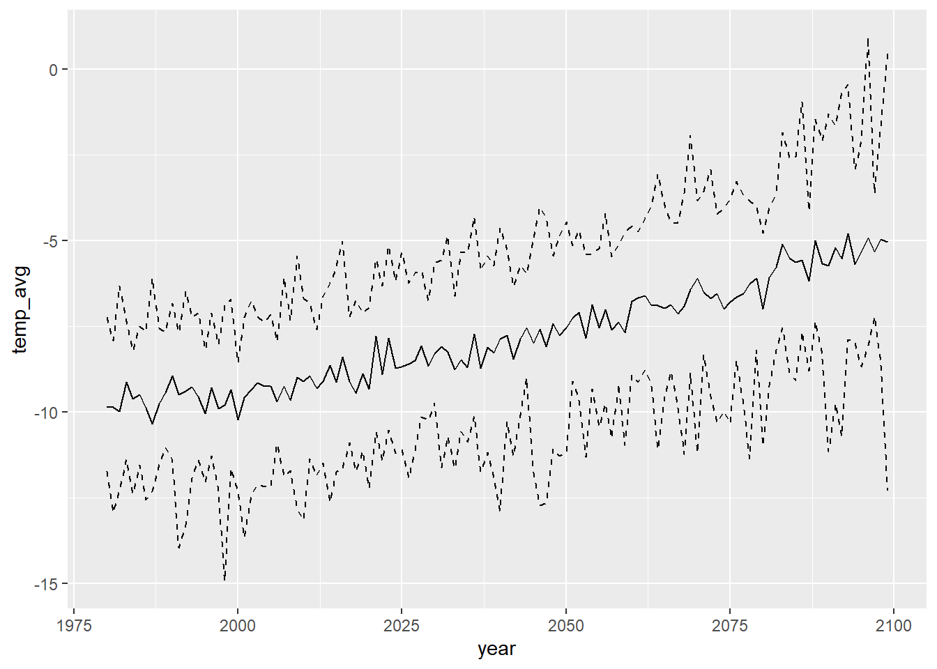

6.1.4 Write out data files

Code

write_csv(dat3, "Data/Derived/SeasonalMeanAirTemp_byGCM_1980-2099.csv")
write_csv(dat_summ, "Data/Derived/SeasonalMeanAirTemp_Summarized_1980-2099.csv")

6.1.5 Read derived data

Code

dat3 <- read_csv("Data/Derived/SeasonalMeanAirTemp_byGCM_1980-2099.csv")
dat_summ <- read_csv("Data/Derived/SeasonalMeanAirTemp_Summarized_1980-2099.csv")

6.2 Compare to observed data

Load NWS air temperature data from Moose, WY

Code

airsum <- read_csv("Data/Derived/AirTemperature_Covariates_BroodYear_1960-2022.csv")

Compare observed data with projections from individual GCMs

Code

ggplot() + 
  geom_line(data = dat3 %>% filter(season == "fal"), aes(x = year, y = temp_mean, group = gcm, colour = gcm)) +
  geom_line(data = airsum %>% filter(site == "moose"), aes(x = broodyr, y = temp_falmean), size = 1.2) + xlim(1960,2100) +
  facet_wrap(~ type, ncol = 2) + theme(legend.position = "none")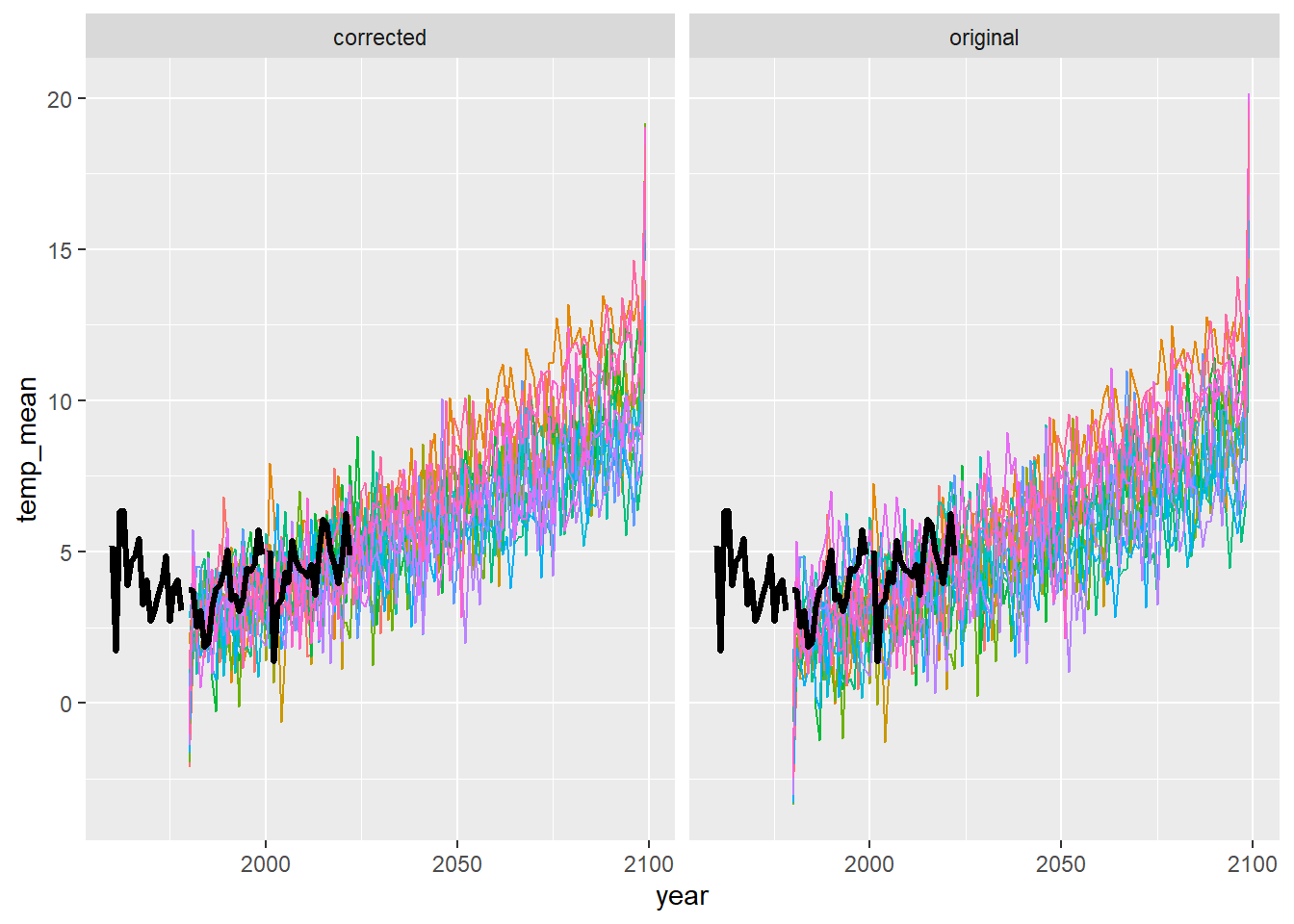

Code

ggplot() + 
  geom_line(data = dat3 %>% filter(season == "win"), aes(x = year, y = temp_mean, group = gcm, colour = gcm)) +
  geom_line(data = airsum %>% filter(site == "moose"), aes(x = broodyr, y = temp_winmean), size = 1.2) + xlim(1960,2100) +
  facet_wrap(~ type, ncol = 2) + theme(legend.position = "none")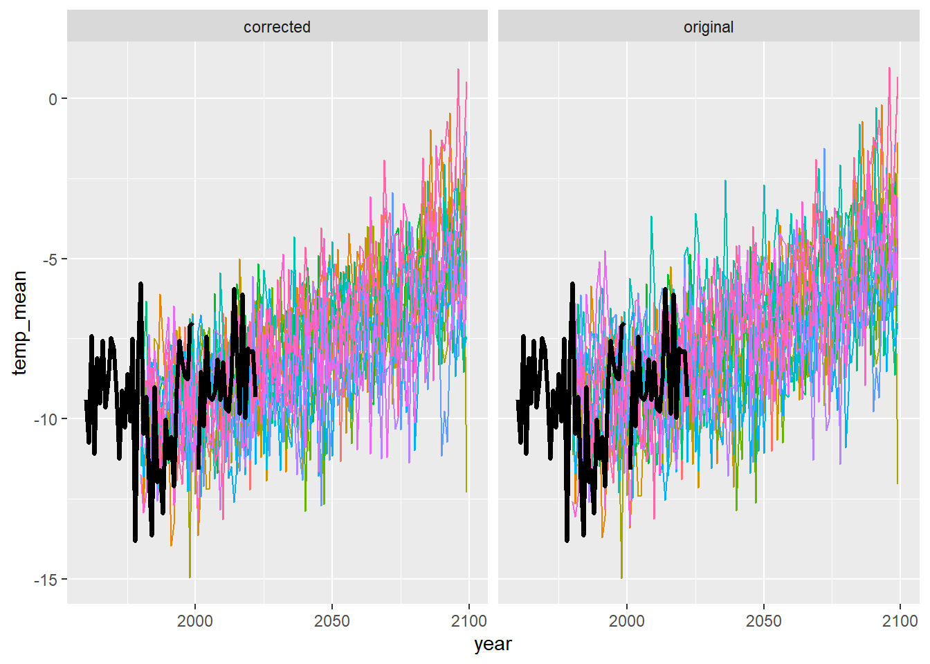

Code

ggplot() + 
  geom_line(data = dat3 %>% filter(season == "spr"), aes(x = year, y = temp_mean, group = gcm, colour = gcm)) +
  geom_line(data = airsum %>% filter(site == "moose"), aes(x = broodyr, y = temp_sprmean), size = 1.2) + xlim(1960,2100) +
  facet_wrap(~ type, ncol = 2) + theme(legend.position = "none")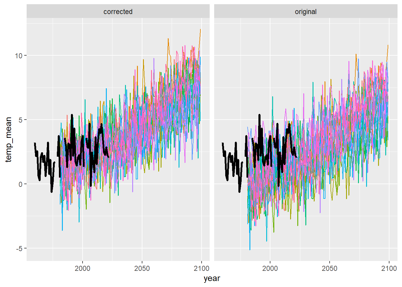

Code

ggplot() + 
  geom_line(data = dat3 %>% filter(season == "sum"), aes(x = year, y = temp_mean, group = gcm, colour = gcm)) +
  geom_line(data = airsum %>% filter(site == "moose"), aes(x = broodyr, y = temp_summean), size = 1.2) + xlim(1960,2100) +
  facet_wrap(~ type, ncol = 2) + theme(legend.position = "none")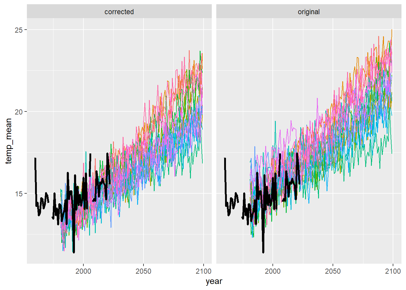

Compare observed data with projections summarized across all GCMs

Code

ggplot() + 
  geom_line(data = dat_summ %>% filter(season == "fal"), aes(x = year, y = temp_avg)) + 
  geom_line(data = dat_summ %>% filter(season == "fal"), aes(x = year, y = temp_min), color = 4) + 
  geom_line(data = dat_summ %>% filter(season == "fal"), aes(x = year, y = temp_max), color = 2) +
  geom_line(data = airsum %>% filter(site == "moose"), aes(x = broodyr, y = temp_falmean), size = 1.2) + xlim(1960,2100) +
  facet_wrap(~ type, ncol = 2) + theme(legend.position = "none")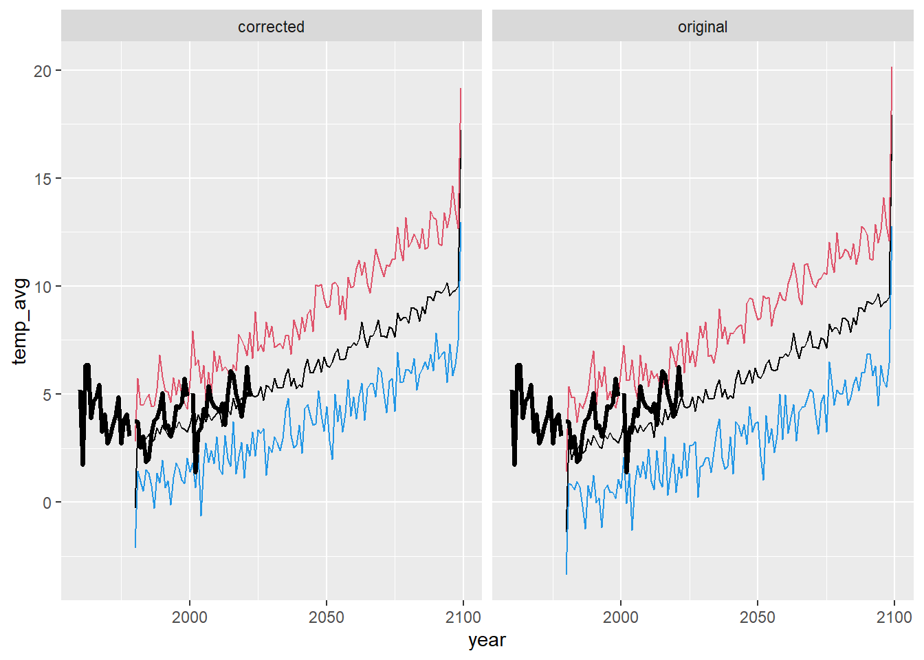

Code

ggplot() + 
  geom_line(data = dat_summ %>% filter(season == "win"), aes(x = year, y = temp_avg)) + 
  geom_line(data = dat_summ %>% filter(season == "win"), aes(x = year, y = temp_min), color = 4) + 
  geom_line(data = dat_summ %>% filter(season == "win"), aes(x = year, y = temp_max), color = 2) +
  geom_line(data = airsum %>% filter(site == "moose"), aes(x = broodyr, y = temp_winmean), size = 1.2) + xlim(1960,2100) +
  facet_wrap(~ type, ncol = 2) + theme(legend.position = "none")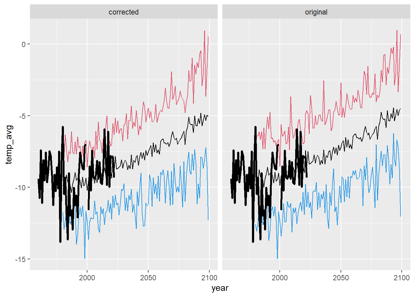

Code

ggplot() + 
  geom_line(data = dat_summ %>% filter(season == "spr"), aes(x = year, y = temp_avg)) + 
  geom_line(data = dat_summ %>% filter(season == "spr"), aes(x = year, y = temp_min), color = 4) + 
  geom_line(data = dat_summ %>% filter(season == "spr"), aes(x = year, y = temp_max), color = 2) +
  geom_line(data = airsum %>% filter(site == "moose"), aes(x = broodyr, y = temp_sprmean), size = 1.2) + xlim(1960,2100) +
  facet_wrap(~ type, ncol = 2) + theme(legend.position = "none")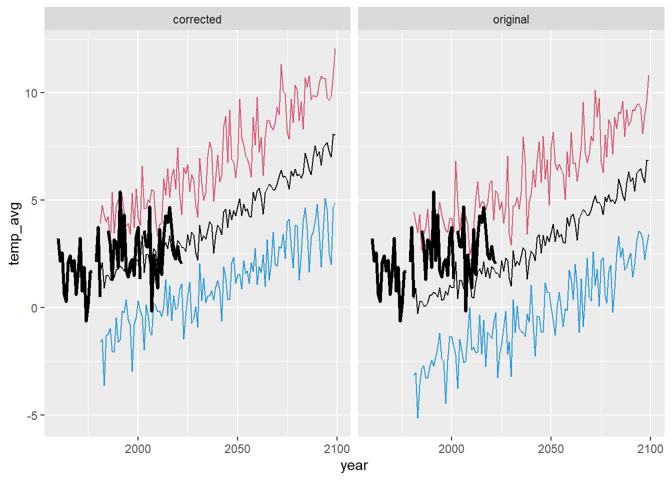

Code

ggplot() + 
  geom_line(data = dat_summ %>% filter(season == "sum"), aes(x = year, y = temp_avg)) + 
  geom_line(data = dat_summ %>% filter(season == "sum"), aes(x = year, y = temp_min), color = 4) + 
  geom_line(data = dat_summ %>% filter(season == "sum"), aes(x = year, y = temp_max), color = 2) +
  geom_line(data = airsum %>% filter(site == "moose"), aes(x = broodyr, y = temp_summean), size = 1.2) + xlim(1960,2100) +
  facet_wrap(~ type, ncol = 2) + theme(legend.position = "none")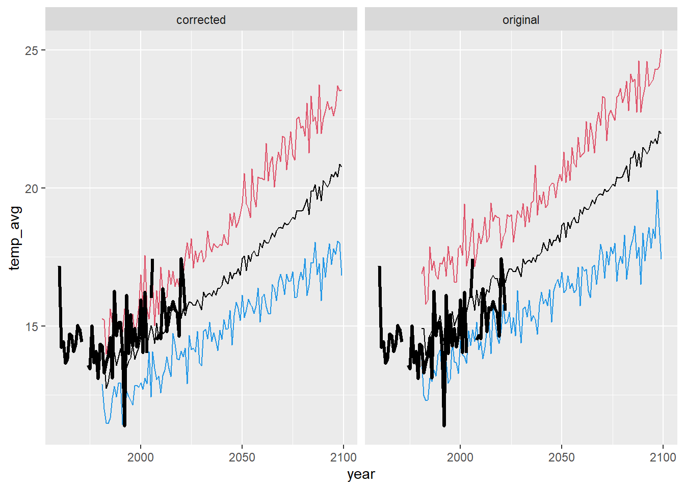

Combined plot for supplementary file

6.3 Exceedance timeline

When will projected seasonal means consistently exceed observed data (w/in the time frame of redd count monitoring)?

Autumn: 2045-2050
Winter: 2083
Spring: 2065
Summer: 2050-2055

Code

maxobs <- airsum %>% filter(site == "moose", broodyr %in% c(1980:2015)) %>% group_by(site) %>% summarise(maxfal = max(temp_falmean, na.rm = T), maxwin = max(temp_winmean, na.rm = T), maxspr = max(temp_sprmean, na.rm = T), maxsum = max(temp_summean, na.rm = T))

dat_summ %>% filter(type == "corrected", season == "fal", temp_avg >= c(maxobs[1,2])) # 2045-2050

# A tibble: 56 × 8
   type      season  year count temp_avg temp_sd temp_min temp_max
   <chr>     <chr>  <dbl> <dbl>    <dbl>   <dbl>    <dbl>    <dbl>
 1 corrected fal     2036    15     6.18   0.994     4.82     7.75
 2 corrected fal     2042    15     6.21   1.11      4.34     7.88
 3 corrected fal     2043    15     6.62   1.23      4.51     8.71
 4 corrected fal     2046    15     6.29   1.62      3.64    10.1 
 5 corrected fal     2047    15     6.63   1.24      5.16    10.0 
 6 corrected fal     2049    15     6.71   1.54      3.29     9.42
 7 corrected fal     2050    15     6.34   1.31      4.42     9.01
 8 corrected fal     2051    15     6.25   1.85      2.83     9.07
 9 corrected fal     2052    15     6.50   1.81      1.99    10.1 
10 corrected fal     2053    15     6.88   1.32      4.98    10.2 
# ℹ 46 more rows

Code

dat_summ %>% filter(type == "corrected", season == "win", temp_avg >= c(maxobs[1,3])) # 2083

# A tibble: 16 × 8
   type      season  year count temp_avg temp_sd temp_min temp_max
   <chr>     <chr>  <dbl> <dbl>    <dbl>   <dbl>    <dbl>    <dbl>
 1 corrected win     2083    15    -5.10    1.62    -7.54   -1.86 
 2 corrected win     2084    15    -5.52    1.92    -8.86   -2.59 
 3 corrected win     2085    15    -5.63    1.84    -9.09   -2.57 
 4 corrected win     2086    15    -5.58    2.06    -7.68   -0.963
 5 corrected win     2088    15    -5.00    1.71    -7.36   -1.47 
 6 corrected win     2089    15    -5.68    1.77    -8.32   -2.08 
 7 corrected win     2090    15    -5.73    2.53   -11.2    -1.29 
 8 corrected win     2091    15    -5.20    2.25    -9.76   -1.64 
 9 corrected win     2092    15    -5.54    2.28   -10.7    -0.699
10 corrected win     2093    15    -4.81    2.05    -7.88   -0.445
11 corrected win     2094    15    -5.70    1.47    -7.95   -2.92 
12 corrected win     2095    15    -5.34    1.99    -8.69   -2.11 
13 corrected win     2096    15    -4.91    2.21    -8.06    0.928
14 corrected win     2097    15    -5.34    1.38    -7.22   -3.64 
15 corrected win     2098    15    -4.97    2.30    -8.54   -1.71 
16 corrected win     2099    15    -5.05    2.97   -12.3     0.517

Code

dat_summ %>% filter(type == "corrected", season == "spr", temp_avg >= c(maxobs[1,4])) # 2065

# A tibble: 37 × 8
   type      season  year count temp_avg temp_sd temp_min temp_max
   <chr>     <chr>  <dbl> <dbl>    <dbl>   <dbl>    <dbl>    <dbl>
 1 corrected spr     2060    15     5.45    2.16     1.08     9.80
 2 corrected spr     2061    15     5.55    1.28     1.89     7.24
 3 corrected spr     2065    15     5.54    1.47     3.15     8.73
 4 corrected spr     2066    15     5.76    2.03     1.27     8.69
 5 corrected spr     2067    15     5.66    1.67     2.06     8.41
 6 corrected spr     2068    15     5.47    1.46     3.52     8.27
 7 corrected spr     2069    15     5.52    1.90     2.03     8.60
 8 corrected spr     2070    15     5.76    1.93     1.93     9.33
 9 corrected spr     2071    15     6.12    1.84     2.84     8.98
10 corrected spr     2072    15     6.40    2.12     2.76    11.3 
# ℹ 27 more rows

Code

dat_summ %>% filter(type == "corrected", season == "sum", temp_avg >= c(maxobs[1,5])) # 2050-2055

# A tibble: 48 × 8
   type      season  year count temp_avg temp_sd temp_min temp_max
   <chr>     <chr>  <dbl> <dbl>    <dbl>   <dbl>    <dbl>    <dbl>
 1 corrected sum     2050    15     17.4   0.891     16.1     19.4
 2 corrected sum     2051    15     17.5   1.48      15.3     20.5
 3 corrected sum     2053    15     17.6   0.926     16.0     19.3
 4 corrected sum     2055    15     17.6   1.37      15.7     20.7
 5 corrected sum     2056    15     17.7   1.17      15.5     19.7
 6 corrected sum     2057    15     17.6   1.06      15.7     19.3
 7 corrected sum     2058    15     17.5   1.27      16.4     20.4
 8 corrected sum     2059    15     18.0   1.23      15.1     20.3
 9 corrected sum     2060    15     17.8   1.33      16.0     20.4
10 corrected sum     2061    15     18.1   1.13      16.2     20.3
# ℹ 38 more rows