7  PASTA

Purpose: use paired air-stream temperature signal analysis to estimate daily groundwater contributions to streamflow

7.1 Data

7.1.1 Site information

siteinfo <- read_csv("C:/Users/jbaldock/OneDrive - DOI/Documents/USGS/EcoDrought/EcoDrought Working/Data/EcoDrought_SiteInformation.csv")
siteinfo_sp <- st_as_sf(siteinfo, coords = c("long", "lat"), crs = 4326)
mapview(siteinfo_sp, zcol = "designation")

Define G-g clusters/sub-basins

siteinfo2 <- siteinfo %>% 
  filter(!site_name %in% c("WoundedBuckCreek", "Brackett Creek", "South River Conway NWIS", 
                           "Shields River nr Livingston NWIS", "North Fork Flathead River NWIS", 
                           "Pacific Creek at Moran NWIS")) %>%
  mutate(designation = ifelse(site_name %in% c("Donner Blitzen River nr Frenchglen NWIS", 
                                               "BigCreekLower", "CoalCreekLower", "McGeeCreekLower", 
                                               "West Brook NWIS", "West Brook 0", 
                                               "Paine Run 10", "Staunton River 10", "Piney River 10", 
                                               "Shields River Valley Ranch", "Shields River ab Smith NWIS", 
                                               "EF Duck Creek be HF",
                                               "Spread Creek Dam"), "big", "little"))

datatable(siteinfo2 %>% 
            arrange(region, basin, subbasin, designation) %>% 
            mutate(lat = round(lat, digits = 2), 
                   long = round(long, digits = 2), 
                   area_sqmi = round(area_sqmi, digits = 2), 
                   elev_ft = round(elev_ft, digits = 0)),
          caption = "EcoDrought monitoring locations and metadata.")

7.1.2 Stream temp

dat <- read_csv("C:/Users/jbaldock/OneDrive - DOI/Documents/USGS/EcoDrought/EcoDrought Working/Data/EcoDrought_FlowTempData_Raw_ECODandNWIS.csv") %>% 
  filter(site_name %in% siteinfo2$site_name) %>% 
  mutate(datetime = floor_date(datetime, unit = "hour")) %>%
  group_by(region, basin, subbasin, site_name, datetime) %>% 
  summarise(tempc = mean(tempc), TempReliability = min(TempReliability), 
            flow = mean(flow), DischargeReliability = min(DischargeReliability)) %>%
  ungroup() %>%
  mutate(flow = ifelse(DischargeReliability == 0, NA, flow)) %>% 
  group_by(region, basin, subbasin, site_name) %>%
  mutate(z_flow = scale(log(flow+0.0001))) %>%
  ungroup()
tz(dat$datetime)

[1] "UTC"

dat

# A tibble: 3,554,087 × 10
   region basin    subbasin  site_name datetime            tempc TempReliability
   <chr>  <chr>    <chr>     <chr>     <dttm>              <dbl>           <dbl>
 1 Flat   Flathead Big Creek Big Cree… 2018-09-10 20:00:00    NA               0
 2 Flat   Flathead Big Creek Big Cree… 2018-09-10 21:00:00    NA               0
 3 Flat   Flathead Big Creek Big Cree… 2018-09-10 22:00:00    NA               0
 4 Flat   Flathead Big Creek Big Cree… 2018-09-10 23:00:00    NA               0
 5 Flat   Flathead Big Creek Big Cree… 2018-09-11 00:00:00    NA               0
 6 Flat   Flathead Big Creek Big Cree… 2018-09-11 01:00:00    NA               0
 7 Flat   Flathead Big Creek Big Cree… 2018-09-11 02:00:00    NA               0
 8 Flat   Flathead Big Creek Big Cree… 2018-09-11 03:00:00    NA               0
 9 Flat   Flathead Big Creek Big Cree… 2018-09-11 04:00:00    NA               0
10 Flat   Flathead Big Creek Big Cree… 2018-09-11 05:00:00    NA               0
# ℹ 3,554,077 more rows
# ℹ 3 more variables: flow <dbl>, DischargeReliability <dbl>, z_flow <dbl[,1]>

7.1.3 Air temp

Apply air temperature data from a single site within/near each sub-basin to all water temperature/flow sites within the same sub-basin. This implicitly assumes that air temperature is homogeneous within each sub-basin, which is an oversimplification, but necessary as we only have air temperature observations at a single site within most sub-basins.

Importantly, SNOTEL data appears to be a reasonable surrogate for in-situ air temperature, at least as shown for the Shields River, Snake River/Spread Creek, and Duck Creek. To maintain consistency across basins (at least in western US) and years where in-situ data is missing, use SNOTEL air temperature data for all western US basins. Note that Duck Creek gets Shields River SNOTEL data, as this was the nearest SNOTEL site, and showed strong concordance with in-situ data. Additionally, using SNOTEL data as a surrogate for in-situ air temperature data may not be as robust in the Donner-Blitzen, where the SNOTEL site is at a considerably higher elevation than the stream monitoring locations.

subbasin	temp_site
West Brook	West Brook Central
Paine Run	Paine Run 10
Staunton River	Staunton River 10
Piney River	Piney River 10
Big Creek	SNOTEL Emery Creek
Coal Creek	SNOTEL Emery Creek
McGee Creek	SNOTEL Emery Creek
Shields River	SNOTEL Porcupine
Duck Creek	SNOTEL Porcupine
Snake River	SNOTEL Base Camp
Donner Blitzen	SNOTEL Silvies

Load air temperature data

# West Brook
airtemp_wb <- read_csv("C:/Users/jbaldock/OneDrive - DOI/Documents/USGS/EcoDrought/EcoDrought Working/Data/Raw Data/Mass/WestBrookCentral_AirTemp_31December2019_to_7July2024.csv")
tz(airtemp_wb$datetime_est) <- "EST"
airtemp_wb$datetime <- with_tz(airtemp_wb$datetime_est, "UTC")
airtemp_wb <- airtemp_wb %>% 
  select(datetime, tempc_air) %>% 
  mutate(datetime = floor_date(datetime, unit = "hour")) %>%
  group_by(datetime) %>% 
  summarise(tempc_air = mean(tempc_air)) %>%
  ungroup() %>%
  mutate(basin = "West Brook", subbasin = "West Brook", source = "SOConte") %>% 
  select(basin, subbasin, source, datetime, tempc_air)


# Shenandoah
airtemp_shen <- read_csv("C:/Users/jbaldock/OneDrive - DOI/Documents/USGS/EcoDrought/EcoDrought Working/Data/Raw data/Virg/Shen_BigG_TempEtc_hourly_UVA.csv") %>%
  rename(tempc_air = airtempc_mean) %>%
  select(site_id, datetime, tempc_air) %>%
  left_join(siteinfo %>% select(site_id, site_name, region, basin, subbasin))
tz(airtemp_shen$datetime) <- "EST"
airtemp_shen$datetime <- with_tz(airtemp_shen$datetime, "UTC")
airtemp_shen <- airtemp_shen %>% 
  mutate(datetime = floor_date(datetime, unit = "hour")) %>%
  group_by(region, basin, subbasin, site_name, datetime) %>% 
  summarise(tempc_air = mean(tempc_air)) %>%
  ungroup() %>%
  select(basin, subbasin, datetime, tempc_air) %>%
  mutate(source = "UVA")


# Flathead
airtemp_flat <- read_csv("C:/Users/jbaldock/OneDrive - DOI/Documents/USGS/EcoDrought/EcoDrought Working/Data/Raw data/Flathead/SNOTEL_469_EmeryCk_4340fasl_AirTemp.csv") %>%
  mutate(datetime = mdy_hm(datetime),
         tempc_air = (tempf - 32) * (5/9),
         basin = "Flathead",
         source = "SNOTEL")
tz(airtemp_flat$datetime) <- "PST" # ALL SNOTEL DATE/TIMES ARE IN PST
airtemp_flat$datetime <- with_tz(airtemp_flat$datetime, "UTC")
airtemp_flat <- airtemp_flat %>% 
  mutate(datetime = floor_date(datetime, unit = "hour")) %>%
  group_by(basin, source, datetime) %>% 
  summarise(tempc_air = mean(tempc_air)) %>%
  ungroup()
airtemp_flat <- bind_rows(airtemp_flat %>% mutate(subbasin = "Big Creek"),
                          airtemp_flat %>% mutate(subbasin = "Coal Creek"),
                          airtemp_flat %>% mutate(subbasin = "McGee Creek"))


# Shields
airtemp_shields <- read_csv("C:/Users/jbaldock/OneDrive - DOI/Documents/USGS/EcoDrought/EcoDrought Working/Data/Raw data/Al-Chokhachy/SNOTEL_700_Porcupine_6480fasl_AirTemp.csv") %>%
  mutate(datetime = mdy_hm(date),
         tempc_air = (tempf - 32) * (5/9),
         basin = "Shields River",
         subbasin = "Shields River",
         source = "SNOTEL")
tz(airtemp_shields$datetime) <- "PST" # ALL SNOTEL DATE/TIMES ARE IN PST
airtemp_shields$datetime <- with_tz(airtemp_shields$datetime, "UTC")
airtemp_shields <- airtemp_shields %>% 
  mutate(datetime = floor_date(datetime, unit = "hour")) %>%
  group_by(basin, subbasin, source, datetime) %>% 
  summarise(tempc_air = mean(tempc_air)) %>%
  ungroup()


# Snake
airtemp_snake <- read_csv("C:/Users/jbaldock/OneDrive - DOI/Documents/USGS/EcoDrought/EcoDrought Working/Data/Raw data/Al-Chokhachy/SNOTEL_314_BaseCampPacific_7040fasl_AirTemp.csv") %>%
  mutate(datetime = mdy_hm(datetime),
         tempc_air = (tempf - 32) * (5/9),
         basin = "Snake River",
         subbasin = "Snake River",
         source = "SNOTEL")
tz(airtemp_snake$datetime) <- "PST" # ALL SNOTEL DATE/TIMES ARE IN PST
airtemp_snake$datetime <- with_tz(airtemp_snake$datetime, "UTC")
airtemp_snake <- airtemp_snake %>% 
  mutate(datetime = floor_date(datetime, unit = "hour")) %>%
  group_by(basin, subbasin, source, datetime) %>% 
  summarise(tempc_air = mean(tempc_air)) %>%
  ungroup()


# Donner-Blitzen
airtemp_db <- read_csv("C:/Users/jbaldock/OneDrive - DOI/Documents/USGS/EcoDrought/EcoDrought Working/Data/Raw data/Oreg/SNOTEL_759_Silvies_7000fasl_AirTemp.csv") %>%
  mutate(datetime = mdy_hm(date),
         tempc_air = (tempf - 32) * (5/9),
         basin = "Donner Blitzen",
         subbasin = "Donner Blitzen",
         source = "SNOTEL")
tz(airtemp_db$datetime) <- "PST" # ALL SNOTEL DATE/TIMES ARE IN PST
airtemp_db$datetime <- with_tz(airtemp_db$datetime, "UTC")
airtemp_db <- airtemp_db %>% 
  mutate(datetime = floor_date(datetime, unit = "hour")) %>%
  group_by(basin, subbasin, source, datetime) %>% 
  summarise(tempc_air = mean(tempc_air)) %>%
  ungroup()

# headers
head(airtemp_wb)

# A tibble: 6 × 5
  basin      subbasin   source  datetime            tempc_air
  <chr>      <chr>      <chr>   <dttm>                  <dbl>
1 West Brook West Brook SOConte 2019-12-31 18:00:00    0.920 
2 West Brook West Brook SOConte 2019-12-31 19:00:00    0.508 
3 West Brook West Brook SOConte 2019-12-31 20:00:00    0.371 
4 West Brook West Brook SOConte 2019-12-31 21:00:00    0.149 
5 West Brook West Brook SOConte 2019-12-31 22:00:00    0.0378
6 West Brook West Brook SOConte 2019-12-31 23:00:00    0.01  

head(airtemp_shen)

# A tibble: 6 × 5
  basin     subbasin  datetime            tempc_air source
  <chr>     <chr>     <dttm>                  <dbl> <chr> 
1 Paine Run Paine Run 2014-10-06 17:00:00      18.6 UVA   
2 Paine Run Paine Run 2014-10-06 18:00:00      19.4 UVA   
3 Paine Run Paine Run 2014-10-06 19:00:00      19.3 UVA   
4 Paine Run Paine Run 2014-10-06 20:00:00      19.4 UVA   
5 Paine Run Paine Run 2014-10-06 21:00:00      18.9 UVA   
6 Paine Run Paine Run 2014-10-06 22:00:00      18.2 UVA   

head(airtemp_flat)

# A tibble: 6 × 5
  basin    source datetime            tempc_air subbasin 
  <chr>    <chr>  <dttm>                  <dbl> <chr>    
1 Flathead SNOTEL 2017-01-01 08:00:00     -5.61 Big Creek
2 Flathead SNOTEL 2017-01-01 09:00:00     -5.61 Big Creek
3 Flathead SNOTEL 2017-01-01 10:00:00     -5.39 Big Creek
4 Flathead SNOTEL 2017-01-01 11:00:00     -5.28 Big Creek
5 Flathead SNOTEL 2017-01-01 12:00:00     -4.72 Big Creek
6 Flathead SNOTEL 2017-01-01 13:00:00     -5.39 Big Creek

head(airtemp_shields)

# A tibble: 6 × 5
  basin         subbasin      source datetime            tempc_air
  <chr>         <chr>         <chr>  <dttm>                  <dbl>
1 Shields River Shields River SNOTEL 2013-01-01 08:00:00     -7.5 
2 Shields River Shields River SNOTEL 2013-01-01 09:00:00     -7.22
3 Shields River Shields River SNOTEL 2013-01-01 10:00:00     -7   
4 Shields River Shields River SNOTEL 2013-01-01 11:00:00     -6.72
5 Shields River Shields River SNOTEL 2013-01-01 12:00:00     -6.22
6 Shields River Shields River SNOTEL 2013-01-01 13:00:00     -5.39

head(airtemp_snake)

# A tibble: 6 × 5
  basin       subbasin    source datetime            tempc_air
  <chr>       <chr>       <chr>  <dttm>                  <dbl>
1 Snake River Snake River SNOTEL 2013-01-01 08:00:00     -13.7
2 Snake River Snake River SNOTEL 2013-01-01 09:00:00     -13.7
3 Snake River Snake River SNOTEL 2013-01-01 10:00:00     -13.6
4 Snake River Snake River SNOTEL 2013-01-01 11:00:00     -13.6
5 Snake River Snake River SNOTEL 2013-01-01 12:00:00     -13.6
6 Snake River Snake River SNOTEL 2013-01-01 13:00:00     -13.6

head(airtemp_db)

# A tibble: 6 × 5
  basin          subbasin       source datetime            tempc_air
  <chr>          <chr>          <chr>  <dttm>                  <dbl>
1 Donner Blitzen Donner Blitzen SNOTEL 2019-01-01 08:00:00     -11.3
2 Donner Blitzen Donner Blitzen SNOTEL 2019-01-01 09:00:00     -11.6
3 Donner Blitzen Donner Blitzen SNOTEL 2019-01-01 10:00:00     -11.7
4 Donner Blitzen Donner Blitzen SNOTEL 2019-01-01 11:00:00     -11.7
5 Donner Blitzen Donner Blitzen SNOTEL 2019-01-01 12:00:00     -11.6
6 Donner Blitzen Donner Blitzen SNOTEL 2019-01-01 13:00:00     -12.3

7.1.3.1 In-situ vs. SNOTEL

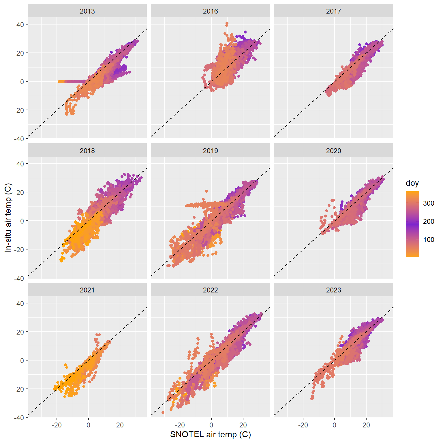
Al-Chokhachy has in-situ air temperature for Duck Creek, the Shields River, and Spread Creek. For Shields and Spread, compare in-situ air temperature measurements with SNOTEL data. Can we justify using SNOTEL data for these and other western basins?

Load in-situ data

# Duck
airtemp_insitu_duck <- read_csv("C:/Users/jbaldock/OneDrive - DOI/Documents/USGS/EcoDrought/EcoDrought Working/Data/Raw data/Al-Chokhachy/duck_air_hourly_021625.csv") %>%
  select(date, time, temperature) %>%
  rename("tempc_air" = "temperature") %>%
  mutate(datetime = as_datetime(paste(date, time, sep = " ")),
         basin = "Duck Creek",
         subbasin = "Duck Creek",
         source = "Al-Ch") %>%
  select(basin, subbasin, source, datetime, tempc_air)
tz(airtemp_insitu_duck$datetime) <- "MST"
airtemp_insitu_duck$datetime <- with_tz(airtemp_insitu_duck$datetime, "UTC")

# Shields
airtemp_insitu_shields <- read_csv("C:/Users/jbaldock/OneDrive - DOI/Documents/USGS/EcoDrought/EcoDrought Working/Data/Raw data/Al-Chokhachy/Shields_air_hourly_021625.csv") %>%
  select(date, time, temperature) %>%
  rename("tempc_air" = "temperature") %>%
  mutate(datetime = as_datetime(paste(date, time, sep = " ")),
         basin = "Shields River",
         subbasin = "Shields River",
         source = "Al-Ch") %>%
  select(basin, subbasin, source, datetime, tempc_air)
tz(airtemp_insitu_shields$datetime) <- "MST"
airtemp_insitu_shields$datetime <- with_tz(airtemp_insitu_shields$datetime, "UTC")

# Spread
airtemp_insitu_spread <- read_csv("C:/Users/jbaldock/OneDrive - DOI/Documents/USGS/EcoDrought/EcoDrought Working/Data/Raw data/Al-Chokhachy/Spread_air_hourly_021625.csv") %>%
  select(date, time, temperature) %>%
  rename("tempc_air" = "temperature") %>%
  mutate(datetime = as_datetime(paste(date, time, sep = " ")),
         basin = "Snake River",
         subbasin = "Snake River",
         source = "Al-Ch") %>%
  select(basin, subbasin, source, datetime, tempc_air)
tz(airtemp_insitu_spread$datetime) <- "MST"
airtemp_insitu_spread$datetime <- with_tz(airtemp_insitu_spread$datetime, "UTC")

airtemp_insitu_duck

# A tibble: 92,400 × 5
   basin      subbasin   source datetime            tempc_air
   <chr>      <chr>      <chr>  <dttm>                  <dbl>
 1 Duck Creek Duck Creek Al-Ch  2014-06-18 07:52:51      5.30
 2 Duck Creek Duck Creek Al-Ch  2014-06-18 08:52:51      4.42
 3 Duck Creek Duck Creek Al-Ch  2014-06-18 09:52:51      3.69
 4 Duck Creek Duck Creek Al-Ch  2014-06-18 10:52:51      3.58
 5 Duck Creek Duck Creek Al-Ch  2014-06-18 11:52:51      3.36
 6 Duck Creek Duck Creek Al-Ch  2014-06-18 12:52:51      3.46
 7 Duck Creek Duck Creek Al-Ch  2014-06-18 13:52:51      4.14
 8 Duck Creek Duck Creek Al-Ch  2014-06-18 14:52:51      5.35
 9 Duck Creek Duck Creek Al-Ch  2014-06-18 15:52:51      7.12
10 Duck Creek Duck Creek Al-Ch  2014-06-18 16:52:51     15.1 
# ℹ 92,390 more rows

airtemp_insitu_shields

# A tibble: 116,979 × 5
   basin         subbasin      source datetime            tempc_air
   <chr>         <chr>         <chr>  <dttm>                  <dbl>
 1 Shields River Shields River Al-Ch  2011-07-09 06:04:56      6.12
 2 Shields River Shields River Al-Ch  2011-07-09 07:04:56      6.24
 3 Shields River Shields River Al-Ch  2011-07-09 08:04:56      5.98
 4 Shields River Shields River Al-Ch  2011-07-09 09:04:56      3.80
 5 Shields River Shields River Al-Ch  2011-07-09 10:04:56      2.13
 6 Shields River Shields River Al-Ch  2011-07-09 11:04:56      1.53
 7 Shields River Shields River Al-Ch  2011-07-09 12:04:56      1.67
 8 Shields River Shields River Al-Ch  2011-07-09 13:04:56      1.31
 9 Shields River Shields River Al-Ch  2011-07-09 14:04:56      2.44
10 Shields River Shields River Al-Ch  2011-07-09 15:04:56      4.95
# ℹ 116,969 more rows

airtemp_insitu_spread

# A tibble: 117,992 × 5
   basin       subbasin    source datetime            tempc_air
   <chr>       <chr>       <chr>  <dttm>                  <dbl>
 1 Snake River Snake River Al-Ch  2011-07-25 20:47:52      30.2
 2 Snake River Snake River Al-Ch  2011-07-25 21:47:52      27.4
 3 Snake River Snake River Al-Ch  2011-07-25 22:47:52      27.2
 4 Snake River Snake River Al-Ch  2011-07-25 23:47:52      27.2
 5 Snake River Snake River Al-Ch  2011-07-26 00:47:52      26.9
 6 Snake River Snake River Al-Ch  2011-07-26 01:47:52      26.5
 7 Snake River Snake River Al-Ch  2011-07-26 02:47:52      23.0
 8 Snake River Snake River Al-Ch  2011-07-26 03:47:52      20.0
 9 Snake River Snake River Al-Ch  2011-07-26 04:47:52      18.3
10 Snake River Snake River Al-Ch  2011-07-26 05:47:52      18.2
# ℹ 117,982 more rows

Shields River

How well does in-situ air temp align with SNOTEL air temp?

cat_shields <- airtemp_shields %>% select(datetime, tempc_air) %>% left_join(airtemp_insitu_shields %>% select(datetime, tempc_air) %>% mutate(datetime = floor_date(datetime, unit = "hour")) %>% rename("tempc_air_alc" = "tempc_air"))
cat_shields %>% dygraph() %>% dyRangeSelector()

cat_shields %>% mutate(doy = yday(datetime), year = year(datetime)) %>% filter(!year %in% c(2014,2015,2024)) %>%
  ggplot(aes(x = tempc_air, y = tempc_air_alc, color = doy)) + 
  geom_point() + geom_abline(intercept = 0, slope = 1, linetype = "dashed") + 
  scale_color_gradient2(midpoint = 182, low = "orange", mid = "purple3", high = "orange") +
  facet_wrap(~year) + xlab("SNOTEL air temp (C)") + ylab("In-situ air temp (C)")

Notes:

• There are a few periods where the in-situ data are clearly wrong, e.g., winter 2013 and November 2016. For the latter, logger appears to be sun affected (in-situ far too warm for August).
• Generally, diel cycles match well. Daily max temps are similar between SNOTEL and in-situ data. However, in-situ daily minimums are far lower than SNOTEL. Could this be located in a cold pit/sink?
• There is a lot of scatter around 1:1 in the scatter plots. Some of this is probably due to slight differences in the time of sensor readings, but most of it is probably due to the issues mentioned above.

Spread Creek

How well does in-situ air temp align with SNOTEL air temp?

cat_spread <- airtemp_snake %>% select(datetime, tempc_air) %>% left_join(airtemp_insitu_spread %>% select(datetime, tempc_air) %>% mutate(datetime = floor_date(datetime, unit = "hour")) %>% rename("tempc_air_alc" = "tempc_air"))
cat_spread %>% dygraph() %>% dyRangeSelector()

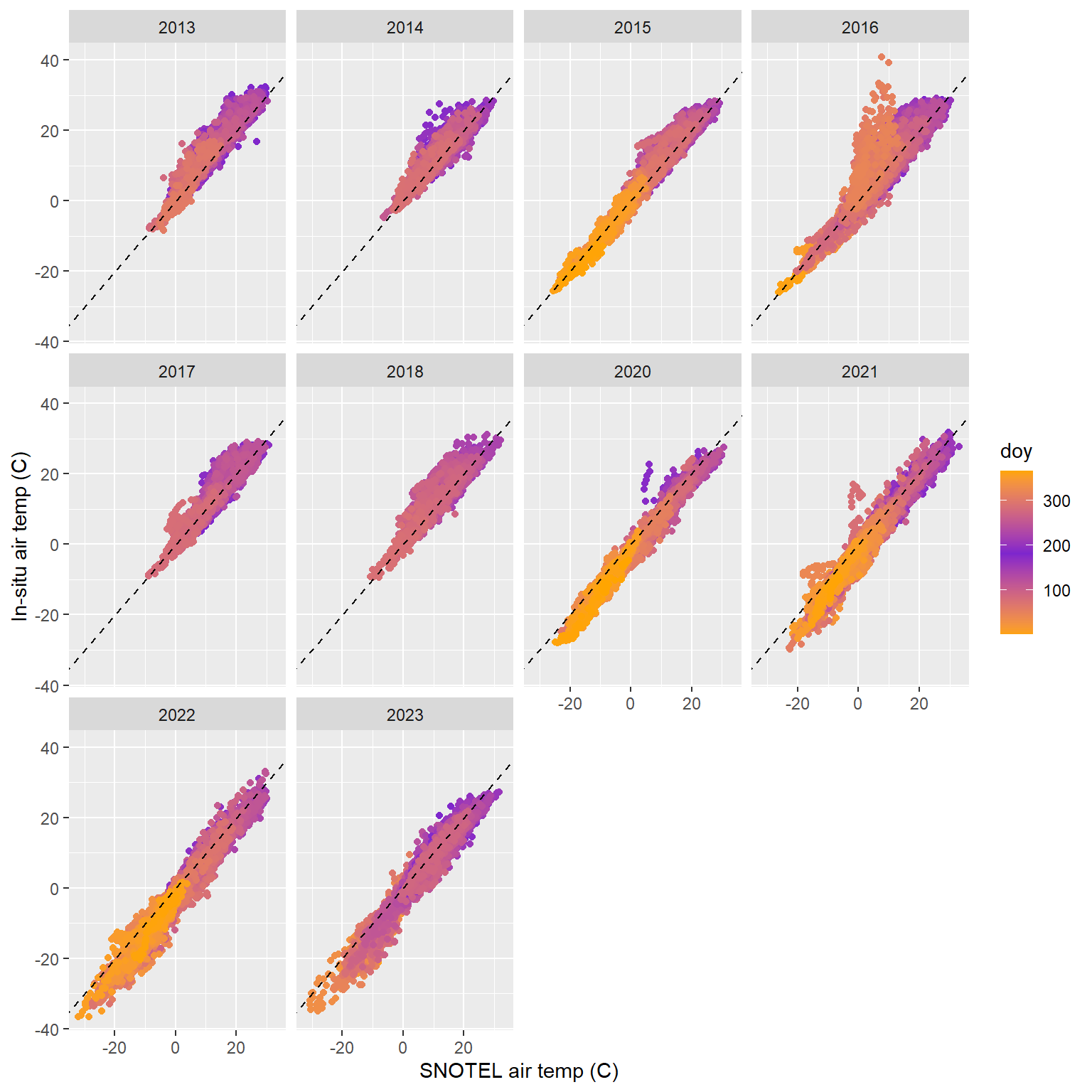
cat_spread %>% mutate(doy = yday(datetime), year = year(datetime)) %>% filter(!year %in% c(2019,2024)) %>%
  ggplot(aes(x = tempc_air, y = tempc_air_alc, color = doy)) + 
  geom_point() + geom_abline(intercept = 0, slope = 1, linetype = "dashed") + 
  scale_color_gradient2(midpoint = 182, low = "orange", mid = "purple3", high = "orange") +
  facet_wrap(~year) + xlab("SNOTEL air temp (C)") + ylab("In-situ air temp (C)")

Notes:

• There is only one apparent period where the in-situ data are clearly wrong: November 2016. In-situ logger appears to be sun affected (in-situ far too warm for August).
• Generally, diel cycles match well (much better than in Shields). Daily max and min temps are similar between SNOTEL and in-situ data, particularly during summer.
• There is some scatter around 1:1 in the scatter plots. Much of this appears to be due to ~45 min lag between sensor readings, but less of the disagreement being driven by actual disagreement between sensor readings.

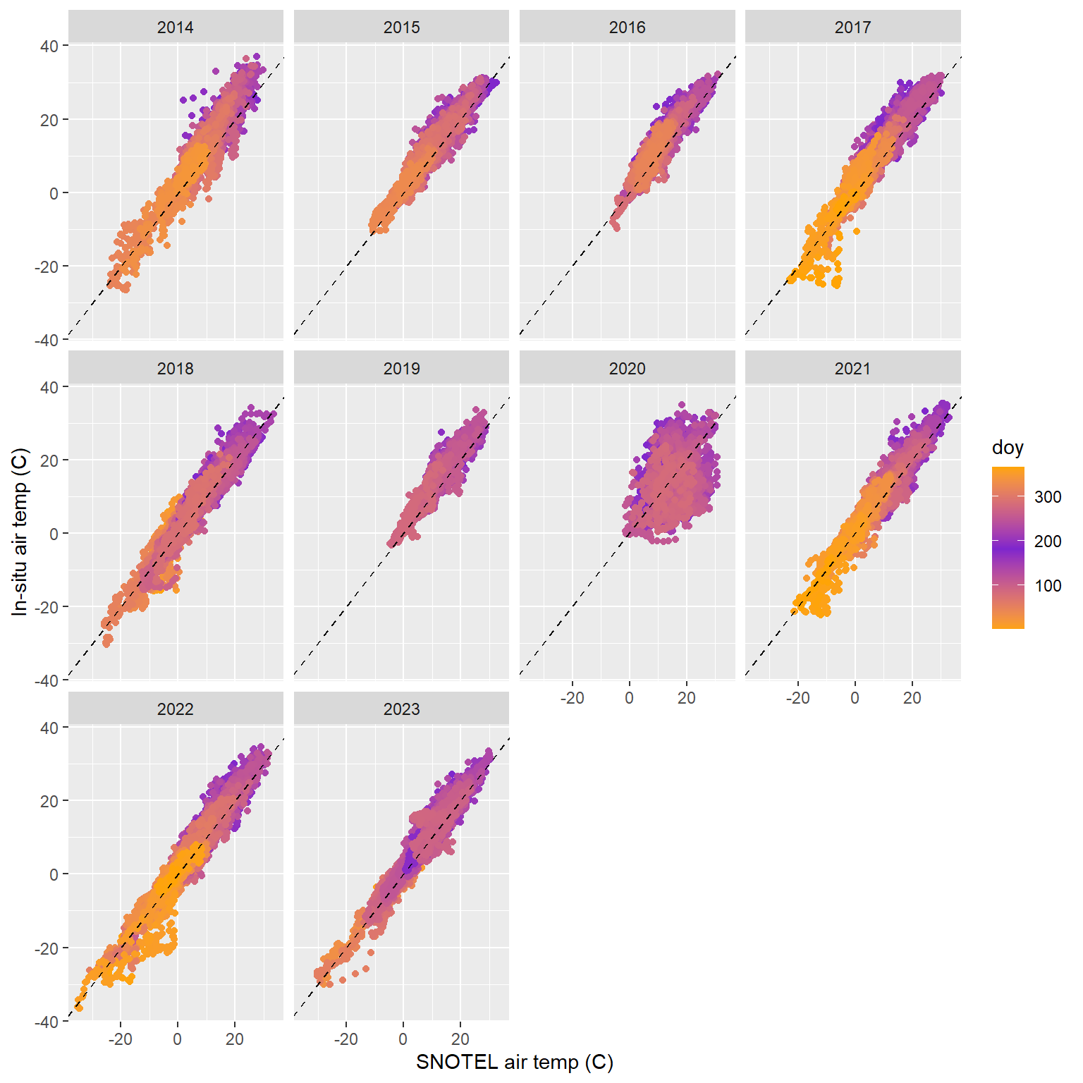
Duck Creek

The closest SNOTEL station is Porcupine in the Shields River basin. How well do these align?

cat_duck <- airtemp_shields %>% select(datetime, tempc_air) %>% left_join(airtemp_insitu_duck %>% select(datetime, tempc_air) %>% mutate(datetime = floor_date(datetime, unit = "hour")) %>% rename("tempc_air_alc" = "tempc_air"))
cat_duck %>% dygraph() %>% dyRangeSelector()

cat_duck %>% mutate(doy = yday(datetime), year = year(datetime)) %>% filter(!year %in% c(2013,2024)) %>%
  ggplot(aes(x = tempc_air, y = tempc_air_alc, color = doy)) + 
  geom_point() + geom_abline(intercept = 0, slope = 1, linetype = "dashed") + 
  scale_color_gradient2(midpoint = 182, low = "orange", mid = "purple3", high = "orange") +
  facet_wrap(~year) + xlab("SNOTEL air temp (C)") + ylab("In-situ air temp (C)")

Notes:

• There is only one apparent period where the in-situ data are clearly wrong: 2020. Date/times are messed up, lack AM/PMs, drives “shotgun” scatter in scatterplot
• Generally, diel cycles match surprisingly well. Daily max and min temps are similar between SNOTEL and in-situ data, particularly during summer. Although in some years daily variability is greater for in-situ data.
• There is some scatter around 1:1 in the scatter plots…on par with what we see in the Snake.

7.1.3.2 Final check

Check time zones (all should be UTC)

tz(airtemp_wb$datetime)

[1] "UTC"

tz(airtemp_shen$datetime)

[1] "UTC"

tz(airtemp_flat$datetime)

[1] "UTC"

tz(airtemp_shields$datetime)

[1] "UTC"

tz(airtemp_snake$datetime)

[1] "UTC"

tz(airtemp_db$datetime)

[1] "UTC"

Bind basin-specific air temp and show unique subbasins

airtemp <- bind_rows(airtemp_wb, airtemp_shen, airtemp_flat, airtemp_shields, airtemp_snake, airtemp_db, airtemp_shields %>% mutate(basin = "Duck Creek", subbasin = "Duck Creek"))
unique(airtemp$subbasin)

 [1] "West Brook"     "Paine Run"      "Piney River"    "Staunton River"
 [5] "Big Creek"      "Coal Creek"     "McGee Creek"    "Shields River" 
 [9] "Snake River"    "Donner Blitzen" "Duck Creek"    

str(airtemp)

tibble [805,771 × 5] (S3: tbl_df/tbl/data.frame)
 $ basin    : chr [1:805771] "West Brook" "West Brook" "West Brook" "West Brook" ...
 $ subbasin : chr [1:805771] "West Brook" "West Brook" "West Brook" "West Brook" ...
 $ source   : chr [1:805771] "SOConte" "SOConte" "SOConte" "SOConte" ...
 $ datetime : POSIXct[1:805771], format: "2019-12-31 18:00:00" "2019-12-31 19:00:00" ...
 $ tempc_air: num [1:805771] 0.9205 0.508 0.3705 0.1487 0.0377 ...

7.1.4 Join data

dat_join <- dat %>% left_join(airtemp)
dat_join

# A tibble: 3,554,087 × 12
   region basin    subbasin  site_name datetime            tempc TempReliability
   <chr>  <chr>    <chr>     <chr>     <dttm>              <dbl>           <dbl>
 1 Flat   Flathead Big Creek Big Cree… 2018-09-10 20:00:00    NA               0
 2 Flat   Flathead Big Creek Big Cree… 2018-09-10 21:00:00    NA               0
 3 Flat   Flathead Big Creek Big Cree… 2018-09-10 22:00:00    NA               0
 4 Flat   Flathead Big Creek Big Cree… 2018-09-10 23:00:00    NA               0
 5 Flat   Flathead Big Creek Big Cree… 2018-09-11 00:00:00    NA               0
 6 Flat   Flathead Big Creek Big Cree… 2018-09-11 01:00:00    NA               0
 7 Flat   Flathead Big Creek Big Cree… 2018-09-11 02:00:00    NA               0
 8 Flat   Flathead Big Creek Big Cree… 2018-09-11 03:00:00    NA               0
 9 Flat   Flathead Big Creek Big Cree… 2018-09-11 04:00:00    NA               0
10 Flat   Flathead Big Creek Big Cree… 2018-09-11 05:00:00    NA               0
# ℹ 3,554,077 more rows
# ℹ 5 more variables: flow <dbl>, DischargeReliability <dbl>, z_flow <dbl[,1]>,
#   source <chr>, tempc_air <dbl>

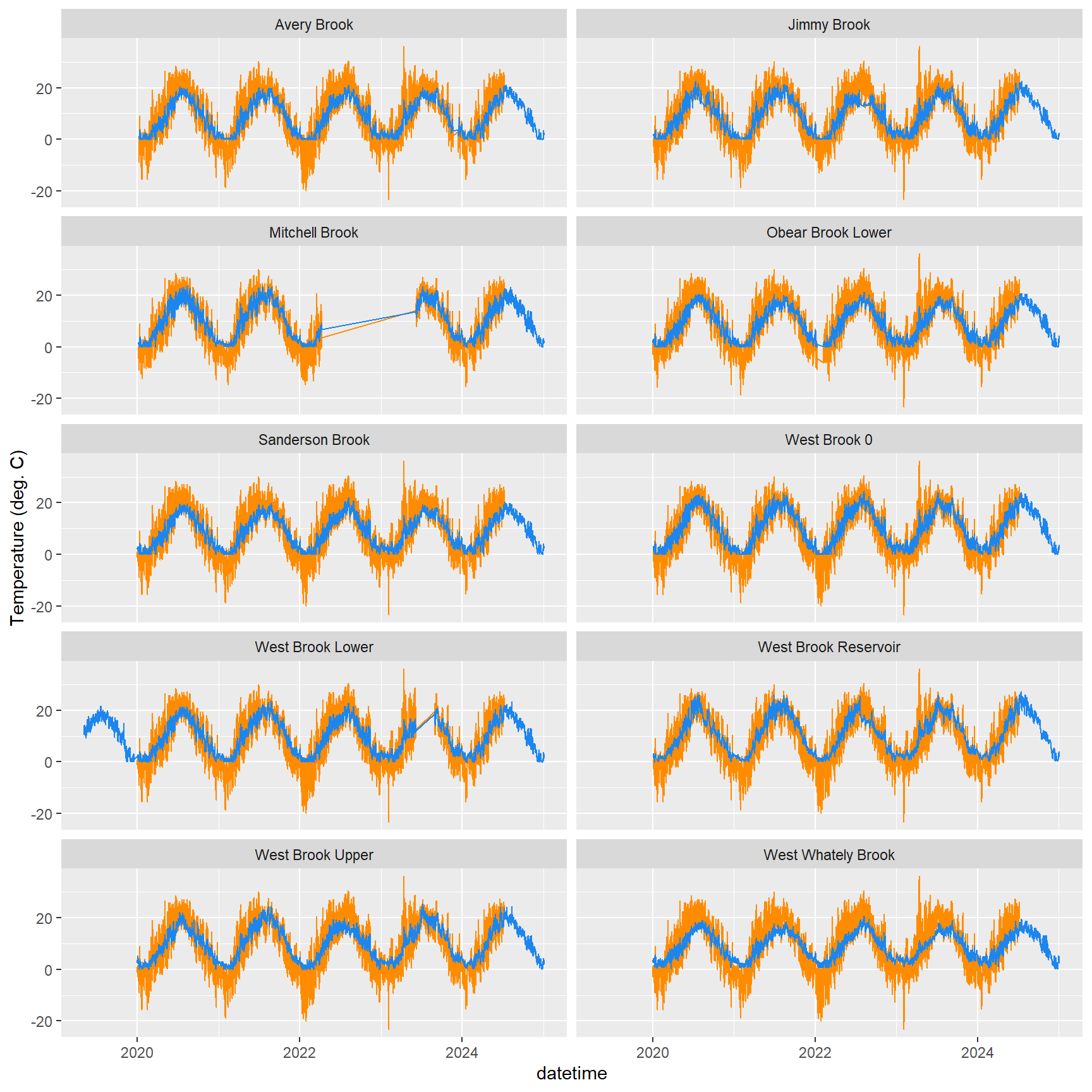
7.1.5 View data

Notes:

• West Brook
  • Mitchell, Obear, and WB Lower have erroneous water temp readings after ~Aug. 31, 2021
  • All WB sites have error in F to C conversion (from Aquarius)
  • Mitchell, Obear, WB0, and WB Lower stream temp signals appear to be shifted forward in time considerably!
• Duck Creek
  • No air temperature data (yet)
• Shields River, Spread Creek, and Donner Blitzen: Should compare SNOTEL air temp data against in-situ/EcoD air temp data, where available

West Brook

Paine Run

Staunton River

Big Creek

Coal Creek

McGee Creek

Shields River

Duck Creek

Snake River

Donner Blitzen

View single site using dyGraphs

mysite <- "SF Spread Creek Lower"
dat_join %>% filter(site_name %in% mysite) %>% select(datetime, tempc, tempc_air) %>% dygraph(main = mysite) %>% dyRangeSelector() %>% dyAxis("y", label = "Stream temp. (deg C)") %>% dyAxis("y2", label = "Air temp. (deg C)") %>% dySeries("tempc", axis = "y", label = "Stream") %>% dySeries("tempc_air", axis = "y2", label = "Air")

7.1.6 Format data for PASTA

dat2 <- dat_join %>% 
  filter(TempReliability == 1) %>%
  mutate(year = year(datetime),
         yday = yday(datetime),
         hour = hour(datetime)) %>%
  rename(airTemperature = tempc_air,
         waterTemperature = tempc) %>%
  select(subbasin, site_name, datetime, year, yday, hour, airTemperature, waterTemperature, flow, z_flow) %>%
  filter(waterTemperature >= 1, waterTemperature <= 25)
range(dat2$waterTemperature)

[1]  1 25

dat2

# A tibble: 2,166,673 × 10
   subbasin  site_name     datetime             year  yday  hour airTemperature
   <chr>     <chr>         <dttm>              <dbl> <dbl> <int>          <dbl>
 1 Big Creek BigCreekLower 2017-09-18 18:00:00  2017   261    18           8.22
 2 Big Creek BigCreekLower 2017-09-18 19:00:00  2017   261    19           8.5 
 3 Big Creek BigCreekLower 2017-09-18 20:00:00  2017   261    20           8.39
 4 Big Creek BigCreekLower 2017-09-18 21:00:00  2017   261    21           7.22
 5 Big Creek BigCreekLower 2017-09-18 22:00:00  2017   261    22           6.89
 6 Big Creek BigCreekLower 2017-09-18 23:00:00  2017   261    23           6.78
 7 Big Creek BigCreekLower 2017-09-19 00:00:00  2017   262     0           6.5 
 8 Big Creek BigCreekLower 2017-09-19 01:00:00  2017   262     1           6.28
 9 Big Creek BigCreekLower 2017-09-19 02:00:00  2017   262     2           5.72
10 Big Creek BigCreekLower 2017-09-19 03:00:00  2017   262     3           5.22
# ℹ 2,166,663 more rows
# ℹ 3 more variables: waterTemperature <dbl>, flow <dbl>, z_flow <dbl[,1]>

7.2 Create functions

7.2.1 Curve fits

Functions to model air and water temperature time series data using sine wave regression:

curve_fit_air <- function(d, minDataLength = 20) {
  # return NAs if not enough data
  if (length(d$airTemperature) < minDataLength) { return(list(model = NA, rSquared = NA)) }
  # convert hours to radians/circular
  d$hour_rad <- d$hour * (2 * pi / 24)
  # starting values
  startAir <- list(A = -1, B = -1, C = mean(d$airTemperature, na.rm = TRUE))
  # run sine wave regression as an NLS model
  modelAir <- tryCatch({
    nlsLM(airTemperature ~ A * sin(hour_rad) + B * cos(hour_rad) + C, data = d, start = startAir)
    }, error = function(e) {
      return(list(model = NA, rSquared = NA))
      })
  # rSquared calculation
  residuals <- residuals(modelAir)
  sst <- sum((d$airTemperature - mean(d$airTemperature))^2)
  ssr <- sum(residuals^2)
  rSquared <- 1 - (ssr / sst)
  # return fitted model object and R2
  return(list(model = modelAir, rSquared = rSquared))
  }

curve_fit_water <- function(d, minDataLength = 20) {
  # return NAs if not enough data
  if (length(d$waterTemperature) < minDataLength) { return(list(model = NA, rSquared = NA)) }
  # convert hours to radians/circular
  d$hour_rad <- d$hour * (2 * pi / 24)
  # starting values
  startWater <- list(A = -1, B = -1, C = mean(d$waterTemperature, na.rm = TRUE))
  # run sine wave regression as an NLS model
  modelWater <- tryCatch({
    nlsLM(waterTemperature ~ A * sin(hour_rad) + B * cos(hour_rad) + C, data = d, start = startWater)
    }, error = function(e) {
      return(list(model = NA, rSquared = NA))
      })
  # rSquared calculation
  residuals <- residuals(modelWater)
  sst <- sum((d$waterTemperature - mean(d$waterTemperature))^2)
  ssr <- sum(residuals^2)
  rSquared <- 1 - (ssr / sst)
  # return fitted model object and R2
  return(list(model = modelWater, rSquared = rSquared))
  }

7.2.2 Extract parameters

Function to extract model parameters from sine wave regression fits:

extract_params <- function(model) {
  if (is.null(model)) {
    return(NULL)
  }

  params <- tryCatch({
    broom.mixed::tidy(model)
  }, error = function(e) {
    NULL
  })

  return(params)
}

7.2.3 Get model parameters

Function to fit sine wave regression models to data and grab amplitude, phase, and mean temperature parameters from fitted model objects:

getParams <- function(dtHOUR, minDataLength = 20) {
  # Models for air temperature
  modelsAir <- dtHOUR %>%
    group_by(site_name, year, yday) %>%
    nest() %>%
    mutate(dataLength = map_dbl(data, ~length(.x$airTemperature))) |>
    filter(dataLength > minDataLength) |> # filter out daily datasets that are too short
    mutate(
      model0 = map(data, curve_fit_air),
      model = map(model0, 'model'),
      rSquared = map(model0, 'rSquared'),
      params = map(model, extract_params)
    ) %>%
    unnest(c(params, rSquared)) |>
    select(-model0, -model, -data) |>
    mutate(tempVar = "air")

  # Models for water temperature
  modelsWater <- dtHOUR %>%
    group_by(site_name, year, yday) %>%
    nest() %>%
    mutate(dataLength = map_dbl(data, ~length(.x$waterTemperature))) |>
    filter(dataLength > minDataLength) |> # filter out daily datasets that are too short
    mutate(
      model0 = map(data, curve_fit_water),
      model = map(model0, 'model'),
      rSquared = map(model0, 'rSquared'),
      params = map(model, extract_params)
    ) %>%
    unnest(c(params, rSquared)) |>
    select(-model0, -model, -data) |>
    mutate(tempVar = "water")

  # Collect air and water models
  models <- bind_rows(modelsAir, modelsWater) |>
    filter(!is.na(term)) |>
    #group_by(site_name, year, yday, tempVar) |>
    select(-std.error, -statistic, -p.value) |> # need to lose these columns so there are no unique values remaining in non-widened cols
    pivot_wider(names_from = term, values_from = estimate)
  
  # Calculate amplitude and phase for air and water data
  params <- models |>
    group_by(site_name, year, yday, tempVar) |>
    mutate(
      amplitude = sqrt(A^2 + B^2),
      phase = ifelse(A < 0,
        12 + (24 / (2 * pi)) * atan(B / A), #switched order of A and B per Tim's email 5/17/24
        (24 / (2 * pi)) * atan(B / A)),
      mean = C
    ) |>
    left_join(
      dtHOUR |> select(site_name, year, yday) |> distinct(), by = c("site_name", "year", "yday")
    ) |>
    ungroup()
  
  # Return amplitude and phase parameters
  return(params)
}

7.2.4 Get derived parameters

Function to calculate amplitude ratio, phase lag, and mean ratio parameters from sine wave regression models fits to daily paired air-stream temperature data:

getAmpPhase <- function(paramsIn) {
  paramsIn |>
    select(site_name, year, yday, tempVar, amplitude, phase, mean, rSquared) |>
    pivot_wider(
      names_from = tempVar,
      values_from = c(amplitude, phase, mean, rSquared)
    ) |>
    select(
      site_name, year, yday,
      starts_with("amplitude"),
      starts_with("phase"),
      starts_with("mean"),
      starts_with("rSquared")
    ) |>
    mutate(
      amplitudeRatio = amplitude_water / amplitude_air,
      phaseLag = ((phase_air - phase_water + 12) %% 24) - 12,#phase_water - phase_air, # Tim's equation for phase lag
      meanRatio = mean_water / mean_air,
      meanOffset = mean_water - mean_air
    )
}

7.2.5 Predictions

Function to predict air or water temperature from fitted models:

getParamsPred <- function(paramsIn) {

  uniqueValues <- paramsIn |>
    distinct(site_name, year, yday, tempVar)

  preds <- crossing(uniqueValues, hour = 0:23) %>%
    left_join(paramsIn, by = c("site_name", "year", "yday", "tempVar")) %>%
    mutate(
      hour_rad = hour * (2 * pi / 24),
      predTemp = A * sin(hour_rad) + B * cos(hour_rad) + C
    )

    return(preds)
 }

7.3 Perform PASTA

7.3.1 Get model parameters

Perform PASTA and write output to file

pasta <- getParams(dtHOUR = dat2)
write_csv(pasta, "C:/Users/jbaldock/OneDrive - DOI/Documents/USGS/EcoDrought/EcoDrought Working/EcoDrought-Analysis/Covariates/pasta_daily_parameters.csv")

Read in

pasta <- read_csv("C:/Users/jbaldock/OneDrive - DOI/Documents/USGS/EcoDrought/EcoDrought Working/EcoDrought-Analysis/Covariates/pasta_daily_parameters.csv")
head(pasta)

# A tibble: 6 × 12
  site_name  year  yday dataLength rSquared tempVar      A     B     C amplitude
  <chr>     <dbl> <dbl>      <dbl>    <dbl> <chr>    <dbl> <dbl> <dbl>     <dbl>
1 BigCreek…  2017   262         24    0.758 air     -0.599  1.26  4.97      1.40
2 BigCreek…  2017   263         24    0.711 air     -0.822  1.62  3.56      1.81
3 BigCreek…  2017   264         24    0.719 air     -1.78   2.16  4.53      2.80
4 BigCreek…  2017   265         24    0.561 air     -1.08   2.26  4.58      2.51
5 BigCreek…  2017   266         24    0.949 air     -1.74   2.49  4.52      3.04
6 BigCreek…  2017   267         24    0.865 air     -4.38   3.23  4.02      5.44
# ℹ 2 more variables: phase <dbl>, mean <dbl>

7.3.2 Get derived parameters

pasta_derived <- getAmpPhase(paramsIn = pasta)
pasta_derived <- pasta_derived %>% mutate(date = parse_date_time(x = paste(year, yday), orders = "yj")) %>% relocate(date, .after = site_name)
head(pasta_derived)

# A tibble: 6 × 16
  site_name     date                 year  yday amplitude_air amplitude_water
  <chr>         <dttm>              <dbl> <dbl>         <dbl>           <dbl>
1 BigCreekLower 2017-09-19 00:00:00  2017   262          1.40           1.04 
2 BigCreekLower 2017-09-20 00:00:00  2017   263          1.81           1.05 
3 BigCreekLower 2017-09-21 00:00:00  2017   264          2.80           1.41 
4 BigCreekLower 2017-09-22 00:00:00  2017   265          2.51           1.22 
5 BigCreekLower 2017-09-23 00:00:00  2017   266          3.04           0.798
6 BigCreekLower 2017-09-24 00:00:00  2017   267          5.44           1.46 
# ℹ 10 more variables: phase_air <dbl>, phase_water <dbl>, mean_air <dbl>,
#   mean_water <dbl>, rSquared_air <dbl>, rSquared_water <dbl>,
#   amplitudeRatio <dbl>, phaseLag <dbl>, meanRatio <dbl>, meanOffset <dbl>

write_csv(pasta_derived, "C:/Users/jbaldock/OneDrive - DOI/Documents/USGS/EcoDrought/EcoDrought Working/EcoDrought-Analysis/Covariates/pasta_derived_parameters_daily.csv")

7.3.3 Predict temperature

Predict air and stream temperature from fitted sine wave regression models and write predictions to file

preds <- getParamsPred(paramsIn = pasta)
preds <- preds %>% mutate(datetime = parse_date_time(x = paste(year, yday, hour), orders = "yjh")) %>% relocate(datetime, .after = site_name) %>% select(site_name, datetime, tempVar, rSquared, predTemp) %>% pivot_wider(names_from = tempVar, values_from = c(predTemp, rSquared))
write_csv(preds, "C:/Users/jbaldock/OneDrive - DOI/Documents/USGS/EcoDrought/EcoDrought Working/EcoDrought-Analysis/Covariates/pasta_predicted_temp.csv")

Read in

preds <- read_csv("C:/Users/jbaldock/OneDrive - DOI/Documents/USGS/EcoDrought/EcoDrought Working/EcoDrought-Analysis/Covariates/pasta_predicted_temp.csv")
tz(preds$datetime) <- "UTC"
head(preds)

# A tibble: 6 × 6
  site_name   datetime            predTemp_air predTemp_water rSquared_air
  <chr>       <dttm>                     <dbl>          <dbl>        <dbl>
1 Avery Brook 2020-01-11 00:00:00        3.76            1.76        0.893
2 Avery Brook 2020-01-11 01:00:00        3.10            1.61        0.893
3 Avery Brook 2020-01-11 02:00:00        2.38            1.48        0.893
4 Avery Brook 2020-01-11 03:00:00        1.67            1.38        0.893
5 Avery Brook 2020-01-11 04:00:00        0.999           1.30        0.893
6 Avery Brook 2020-01-11 05:00:00        0.423           1.27        0.893
# ℹ 1 more variable: rSquared_water <dbl>

7.4 Explore PASTA output

Add mean daily flow to derived PASTA metrics (z-scored by site)

dat3 <- dat2 %>% 
  mutate(date = as_date(datetime)) %>% 
  group_by(site_name, date) %>% 
  summarize(flow = mean(flow, na.rm = TRUE), z_flow = mean(z_flow, na.rm = TRUE))
pasta_derived <- pasta_derived %>% left_join(dat3)
head(pasta_derived)

# A tibble: 6 × 18
  site_name     date                 year  yday amplitude_air amplitude_water
  <chr>         <dttm>              <dbl> <dbl>         <dbl>           <dbl>
1 BigCreekLower 2017-09-19 00:00:00  2017   262          1.40           1.04 
2 BigCreekLower 2017-09-20 00:00:00  2017   263          1.81           1.05 
3 BigCreekLower 2017-09-21 00:00:00  2017   264          2.80           1.41 
4 BigCreekLower 2017-09-22 00:00:00  2017   265          2.51           1.22 
5 BigCreekLower 2017-09-23 00:00:00  2017   266          3.04           0.798
6 BigCreekLower 2017-09-24 00:00:00  2017   267          5.44           1.46 
# ℹ 12 more variables: phase_air <dbl>, phase_water <dbl>, mean_air <dbl>,
#   mean_water <dbl>, rSquared_air <dbl>, rSquared_water <dbl>,
#   amplitudeRatio <dbl>, phaseLag <dbl>, meanRatio <dbl>, meanOffset <dbl>,
#   flow <dbl>, z_flow <dbl>

View all sites

unique(pasta_derived$site_name)

 [1] "BigCreekLower"                          
 [2] "BigCreekMiddle"                         
 [3] "BigCreekUpper"                          
 [4] "HallowattCreekLower"                    
 [5] "LangfordCreekLower"                     
 [6] "LangfordCreekUpper"                     
 [7] "NicolaCreek"                            
 [8] "SkookoleelCreek"                        
 [9] "WernerCreek"                            
[10] "CoalCreekHeadwaters"                    
[11] "CoalCreekLower"                         
[12] "CoalCreekMiddle"                        
[13] "CoalCreekNorth"                         
[14] "CycloneCreekLower"                      
[15] "CycloneCreekMiddle"                     
[16] "CycloneCreekUpper"                      
[17] "McGeeCreekLower"                        
[18] "McGeeCreekTrib"                         
[19] "McGeeCreekUpper"                        
[20] "Avery Brook"                            
[21] "Jimmy Brook"                            
[22] "Mitchell Brook"                         
[23] "Obear Brook Lower"                      
[24] "Sanderson Brook"                        
[25] "West Brook 0"                           
[26] "West Brook Lower"                       
[27] "West Brook Reservoir"                   
[28] "West Brook Upper"                       
[29] "West Whately Brook"                     
[30] "Donner Blitzen River nr Frenchglen NWIS"
[31] "Donner Blitzen ab Fish NWIS"            
[32] "Donner Blitzen ab Indian NWIS"          
[33] "Donner Blitzen nr Burnt Car NWIS"       
[34] "Fish Creek NWIS"                        
[35] "Indian Creek NWIS"                      
[36] "Little Blizten River NWIS"              
[37] "Paine Run 01"                           
[38] "Paine Run 02"                           
[39] "Paine Run 06"                           
[40] "Paine Run 07"                           
[41] "Paine Run 08"                           
[42] "Paine Run 10"                           
[43] "Piney River 10"                         
[44] "Staunton River 02"                      
[45] "Staunton River 03"                      
[46] "Staunton River 06"                      
[47] "Staunton River 07"                      
[48] "Staunton River 09"                      
[49] "Staunton River 10"                      
[50] "EF Duck Creek ab HF"                    
[51] "EF Duck Creek be HF"                    
[52] "Henrys Fork"                            
[53] "Buck Creek"                             
[54] "Crandall Creek"                         
[55] "Deep Creek"                             
[56] "Dugout Creek"                           
[57] "Dugout Creek NWIS"                      
[58] "Lodgepole Creek"                        
[59] "Shields River Valley Ranch"             
[60] "Shields River ab Dugout"                
[61] "Shields River ab Smith NWIS"            
[62] "Grizzly Creek"                          
[63] "Grouse Creek"                           
[64] "Leidy Creek Mouth"                      
[65] "Leidy Creek Mouth NWIS"                 
[66] "Leidy Creek Upper"                      
[67] "NF Spread Creek Lower"                  
[68] "NF Spread Creek Upper"                  
[69] "Rock Creek"                             
[70] "SF Spread Creek Lower"                  
[71] "SF Spread Creek Lower NWIS"             
[72] "SF Spread Creek Upper"                  
[73] "Spread Creek Dam"                       

7.4.1 Single site

Generate interactive time series plots of PASTA output for a single focal site

Set focal site

focal_site <- "Leidy Creek Mouth NWIS"
focal_site

[1] "Leidy Creek Mouth NWIS"

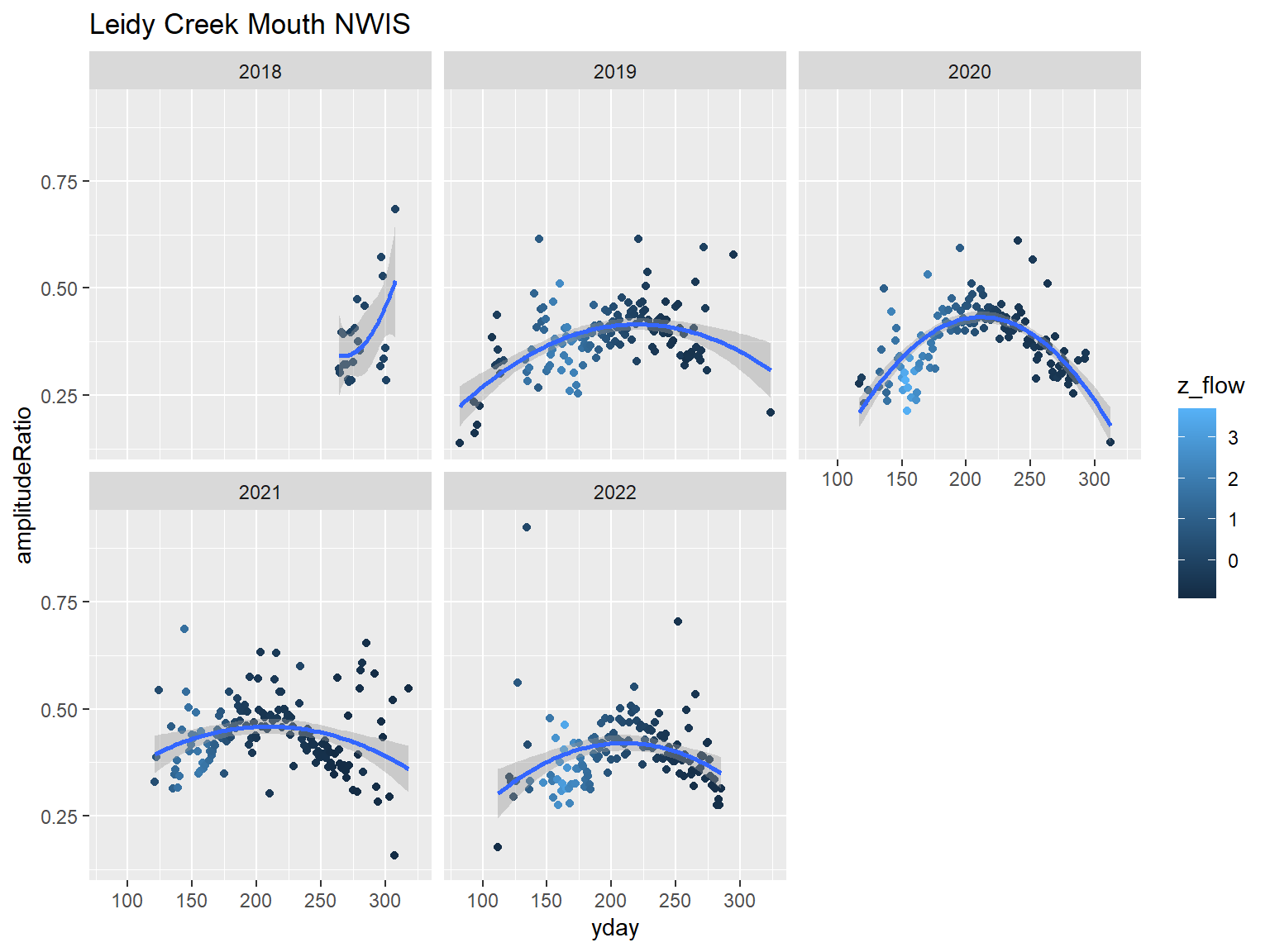
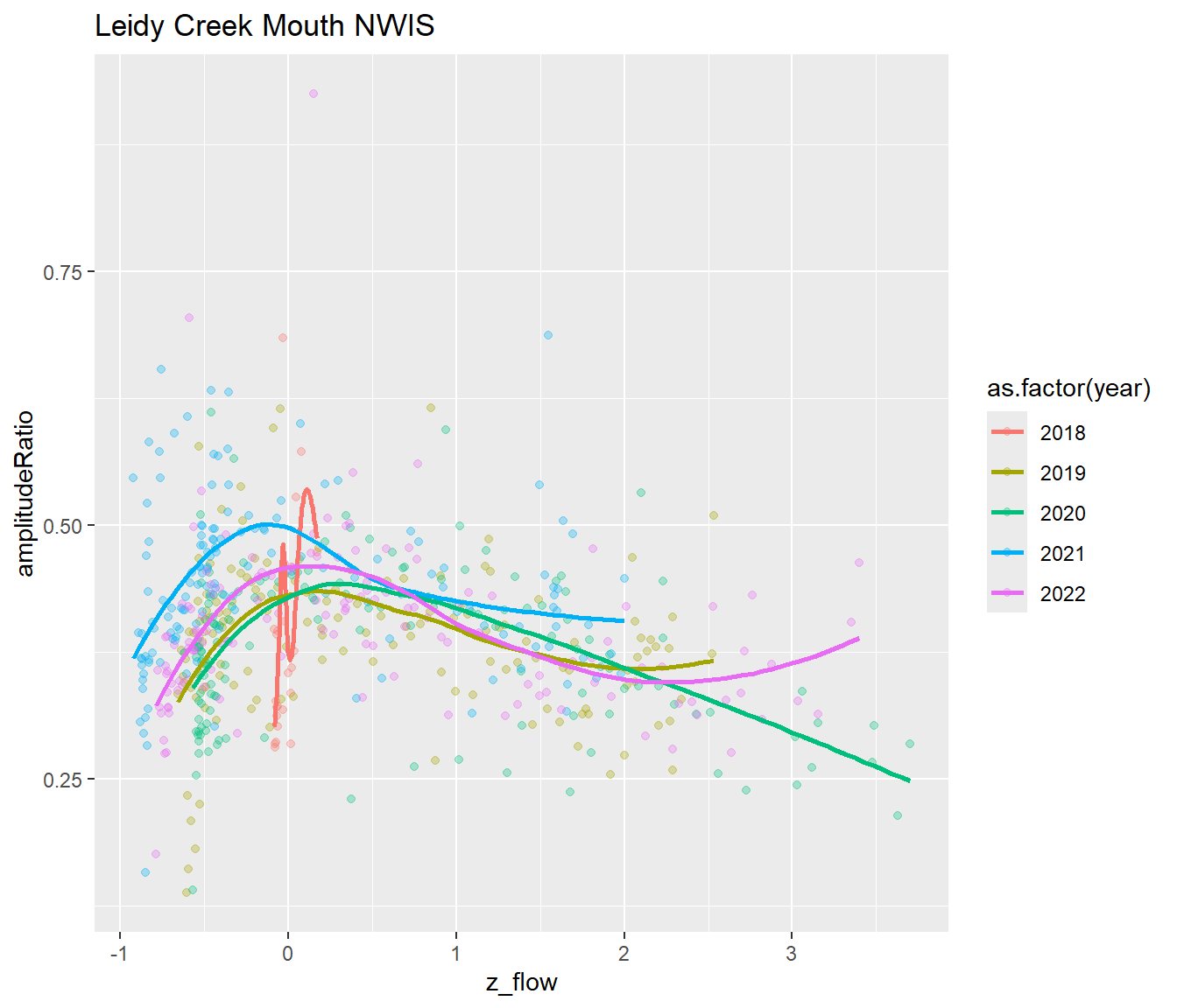
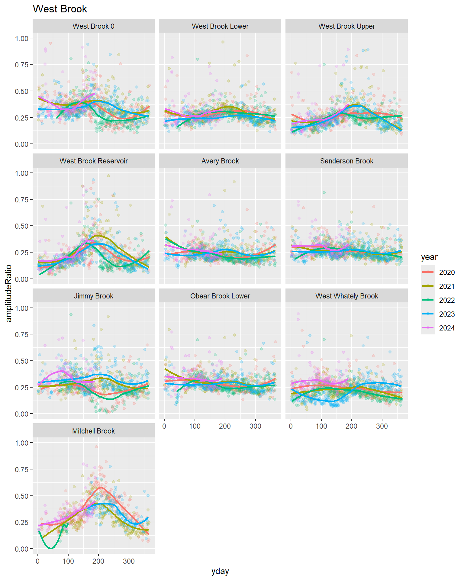
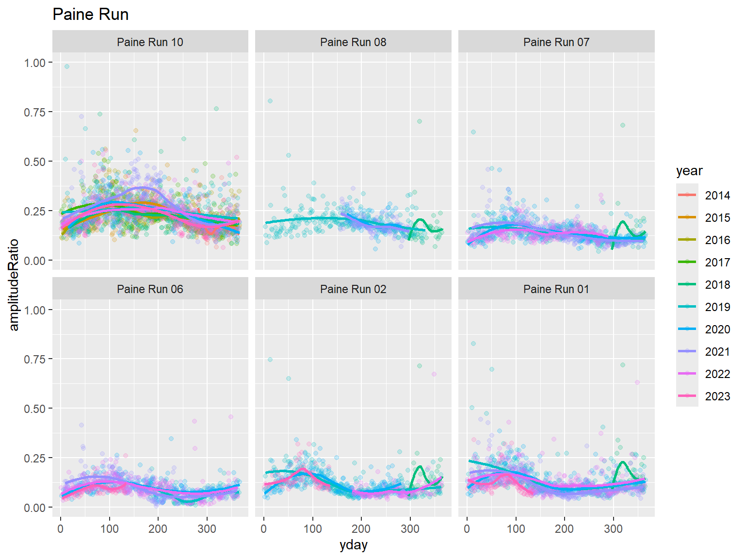
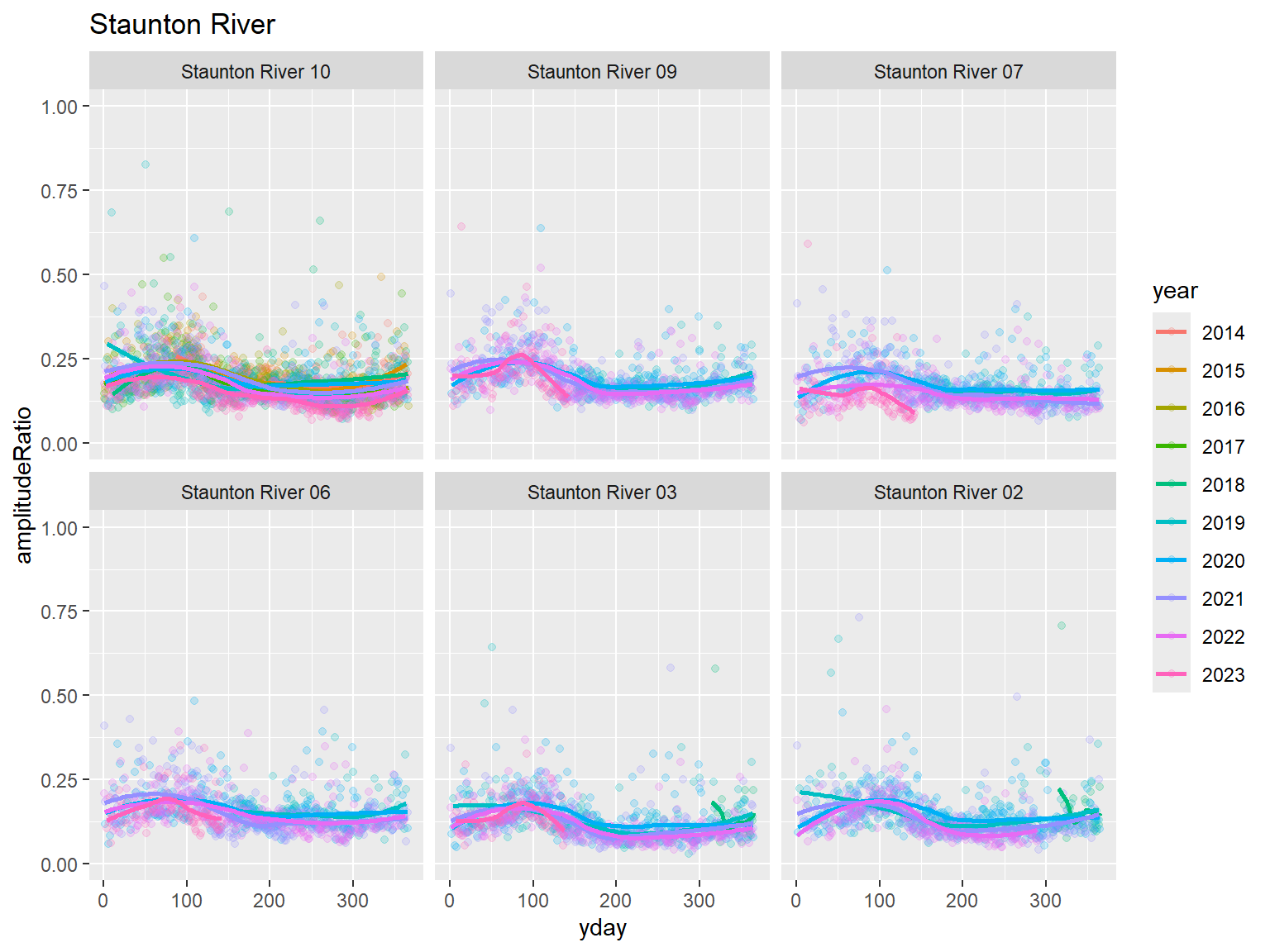
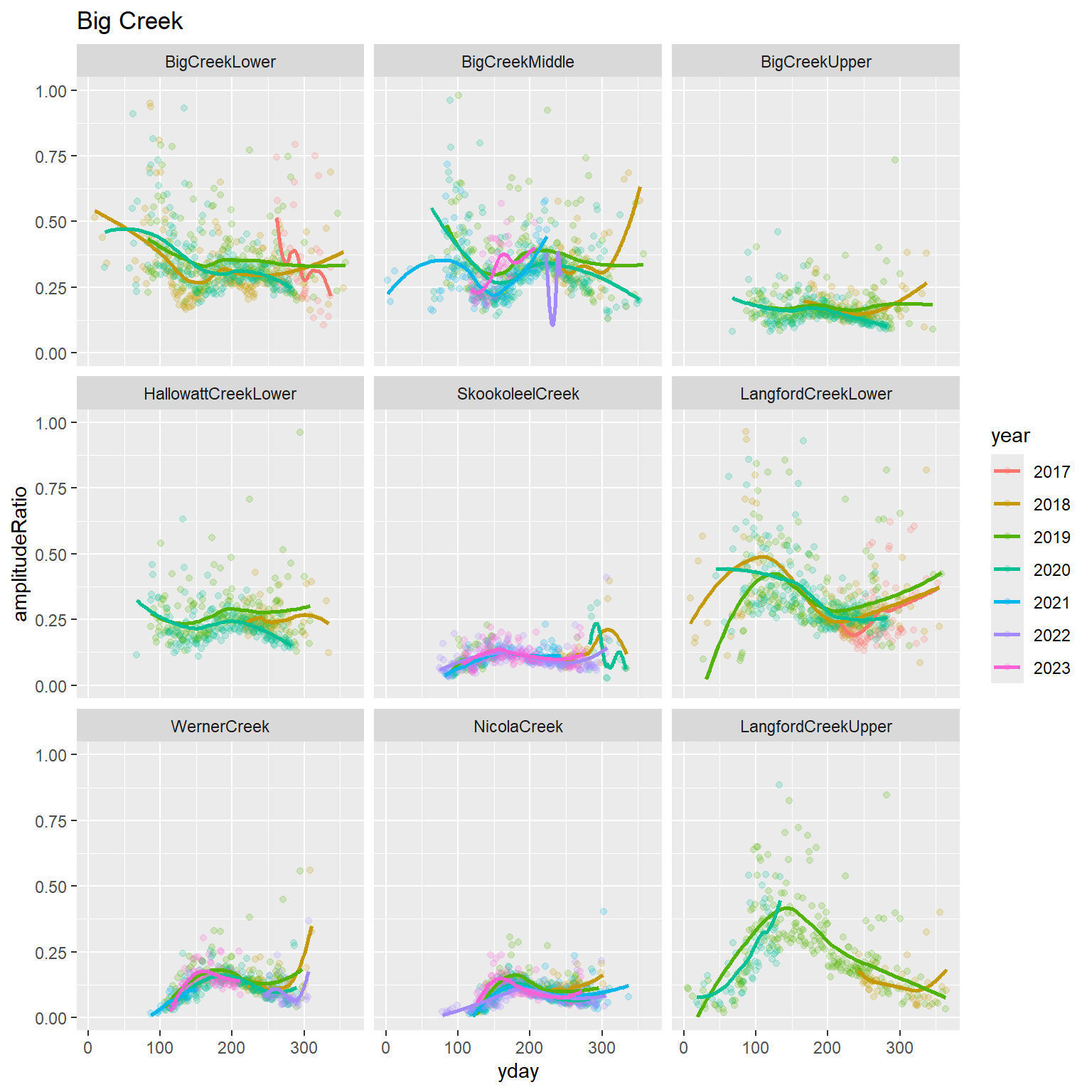
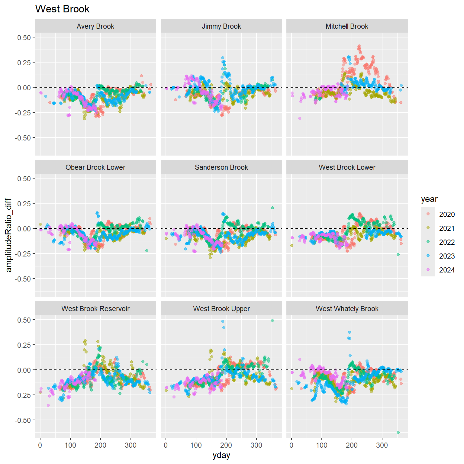
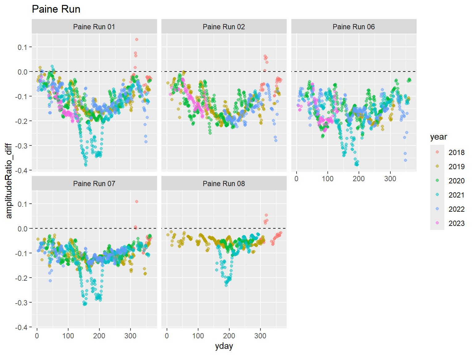
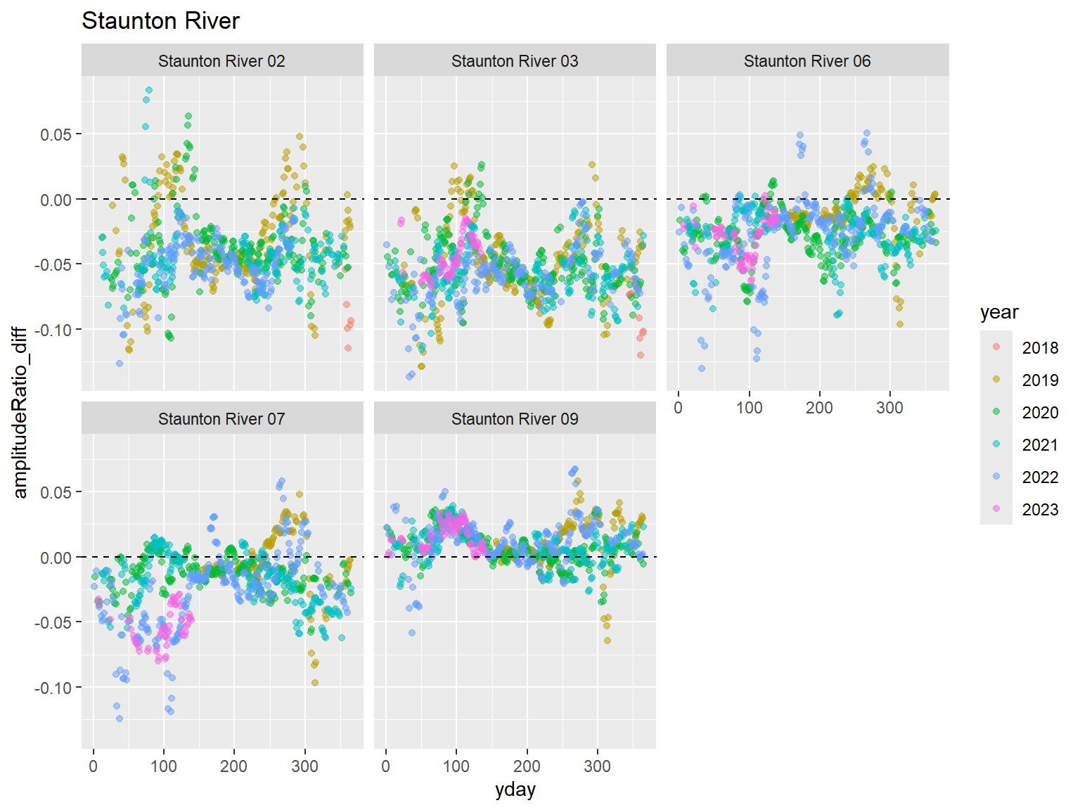
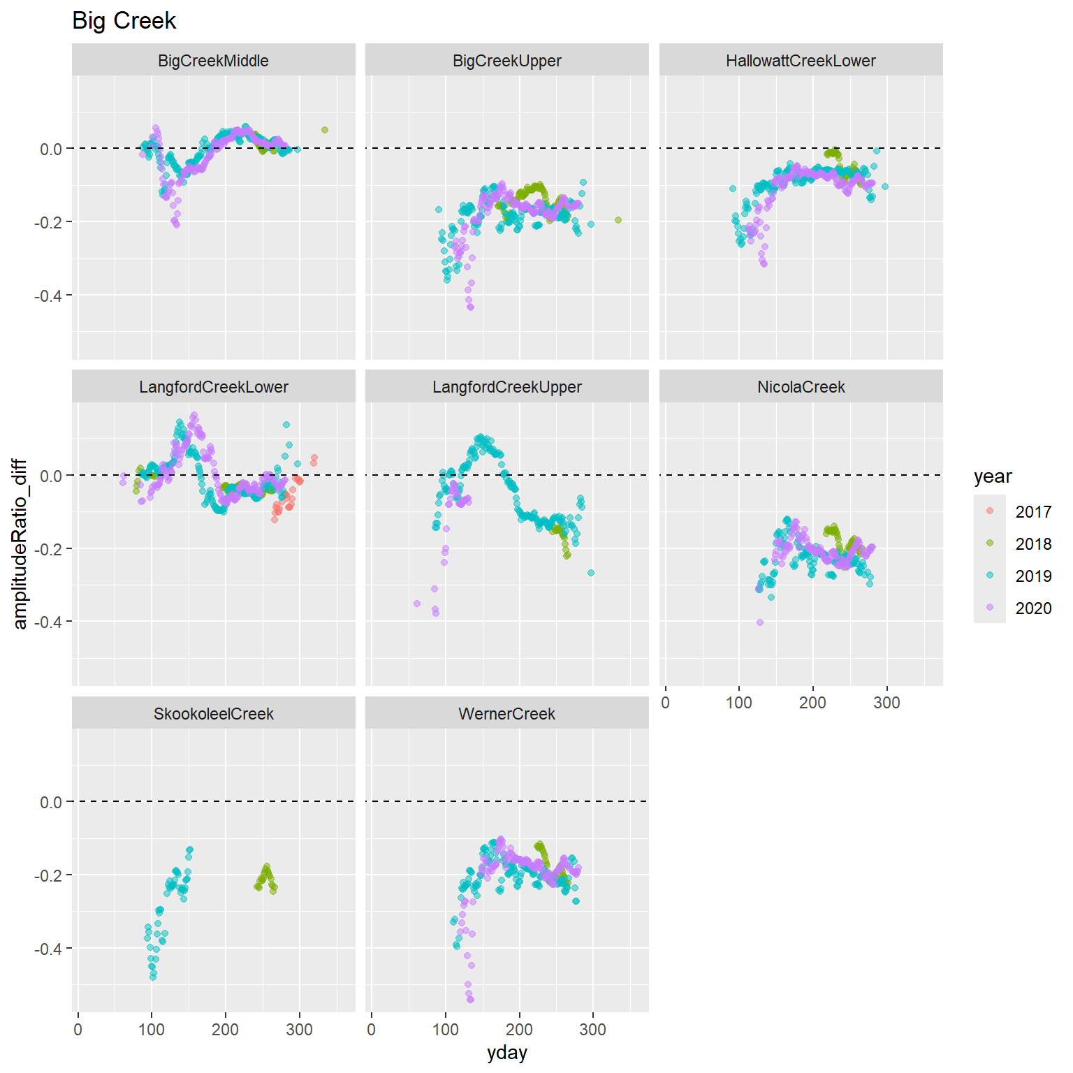
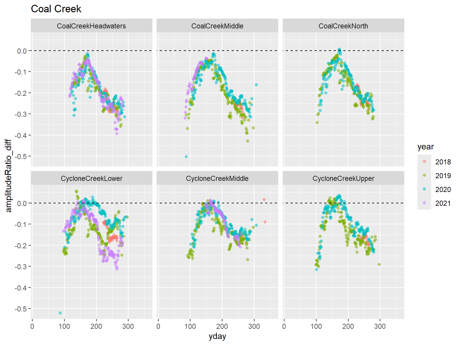
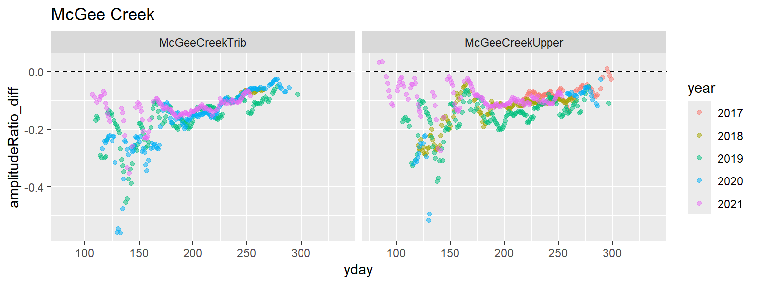
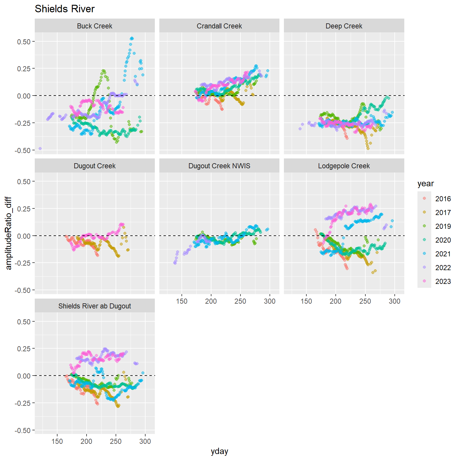
7.4.1.1 Amplitude ratio

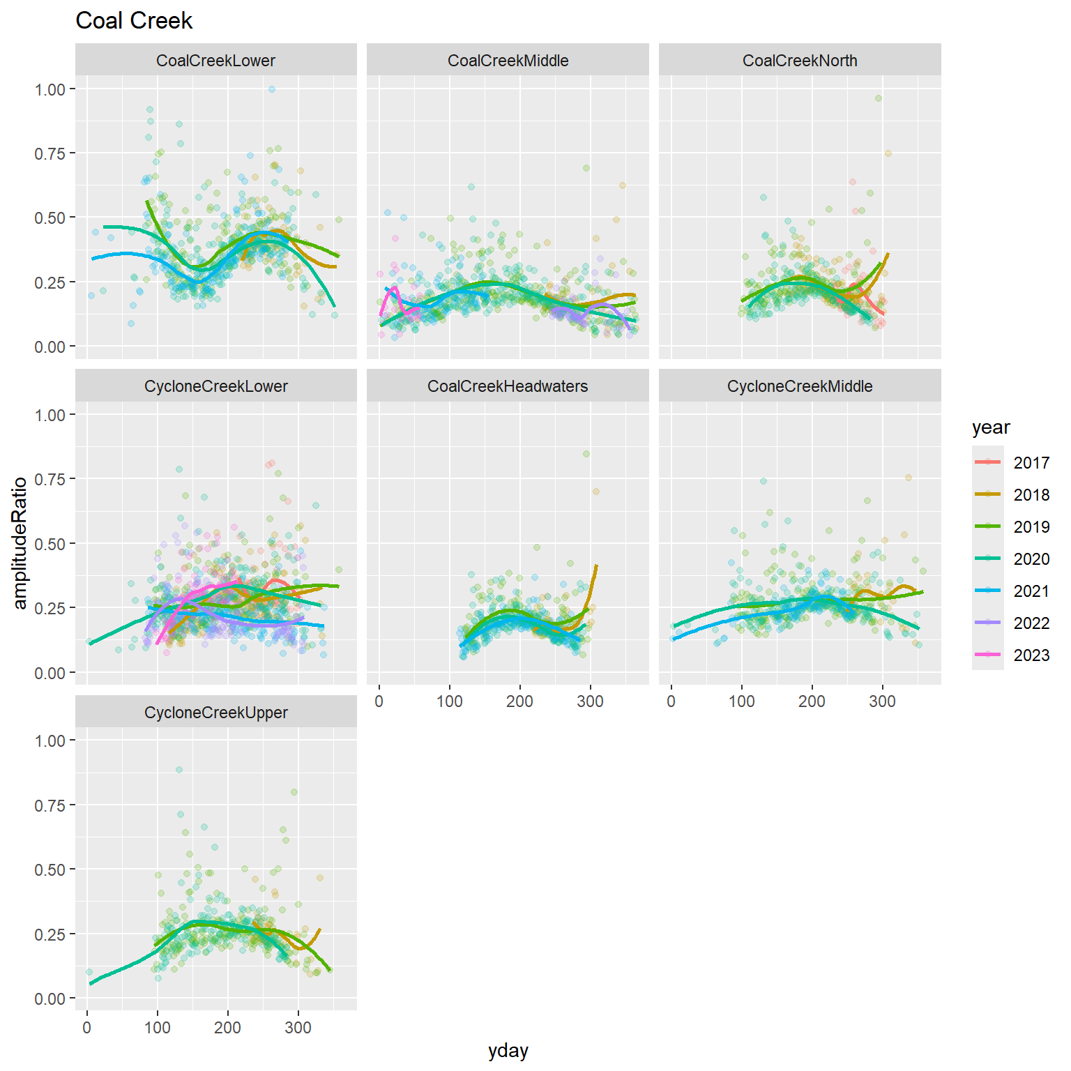
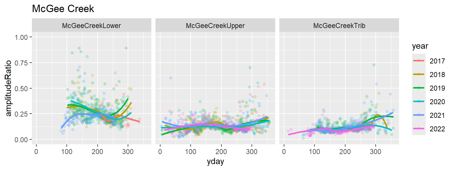
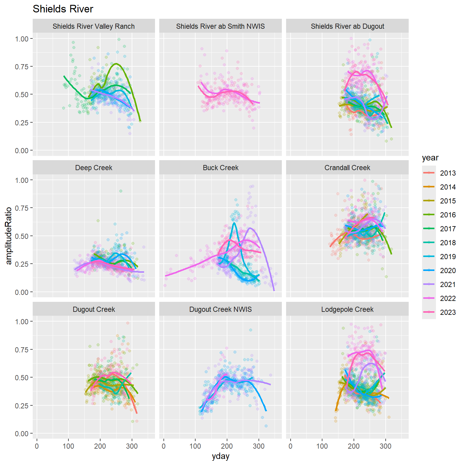
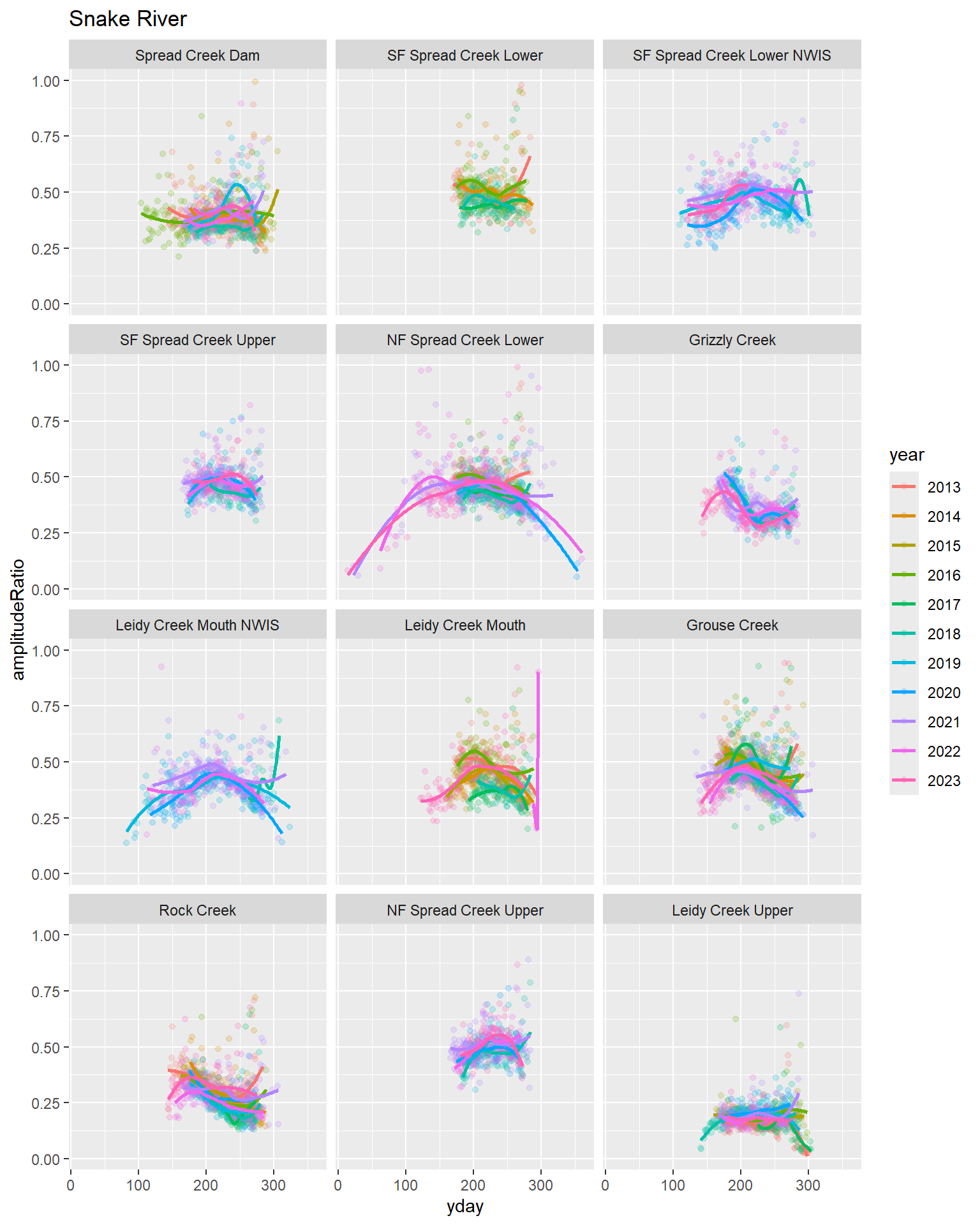
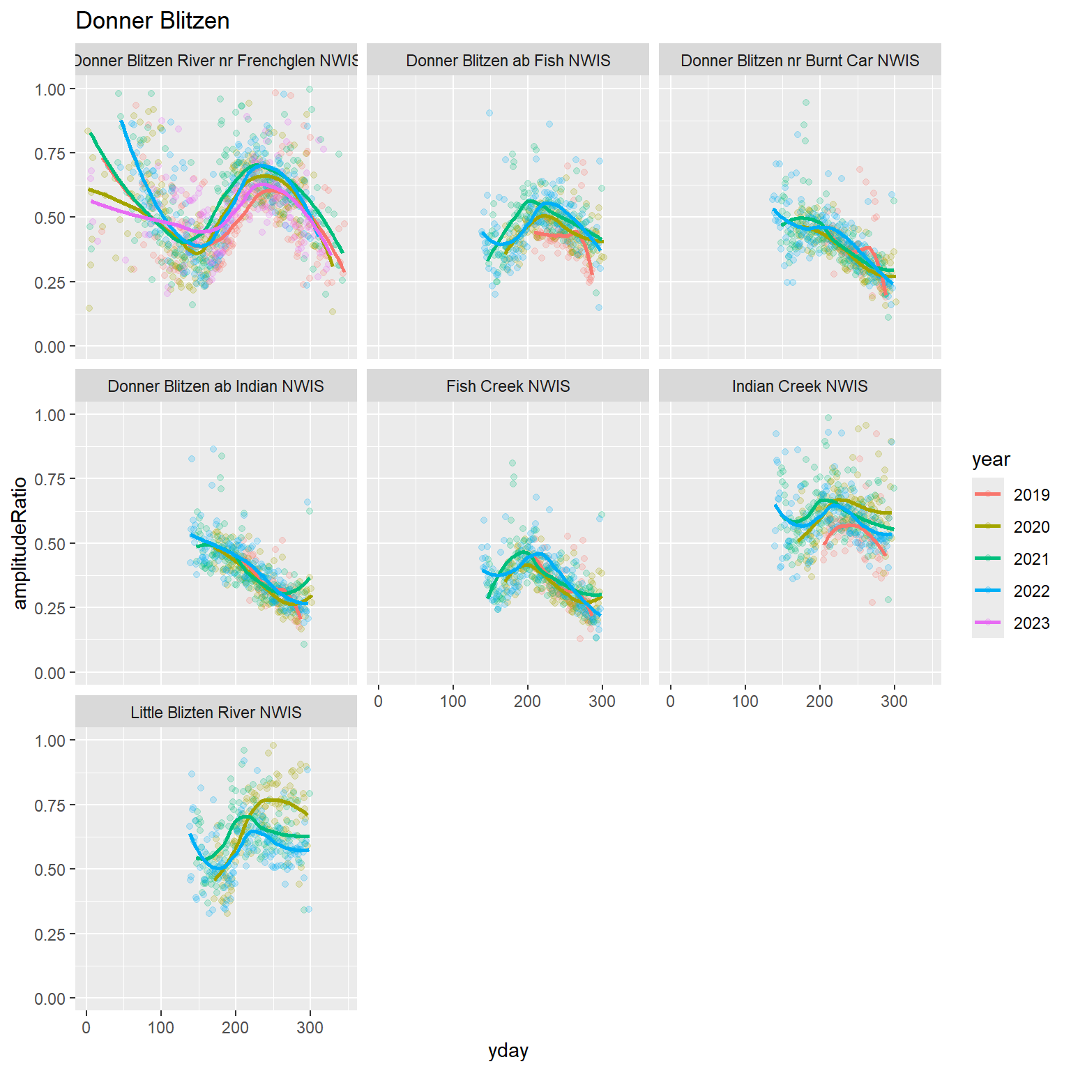
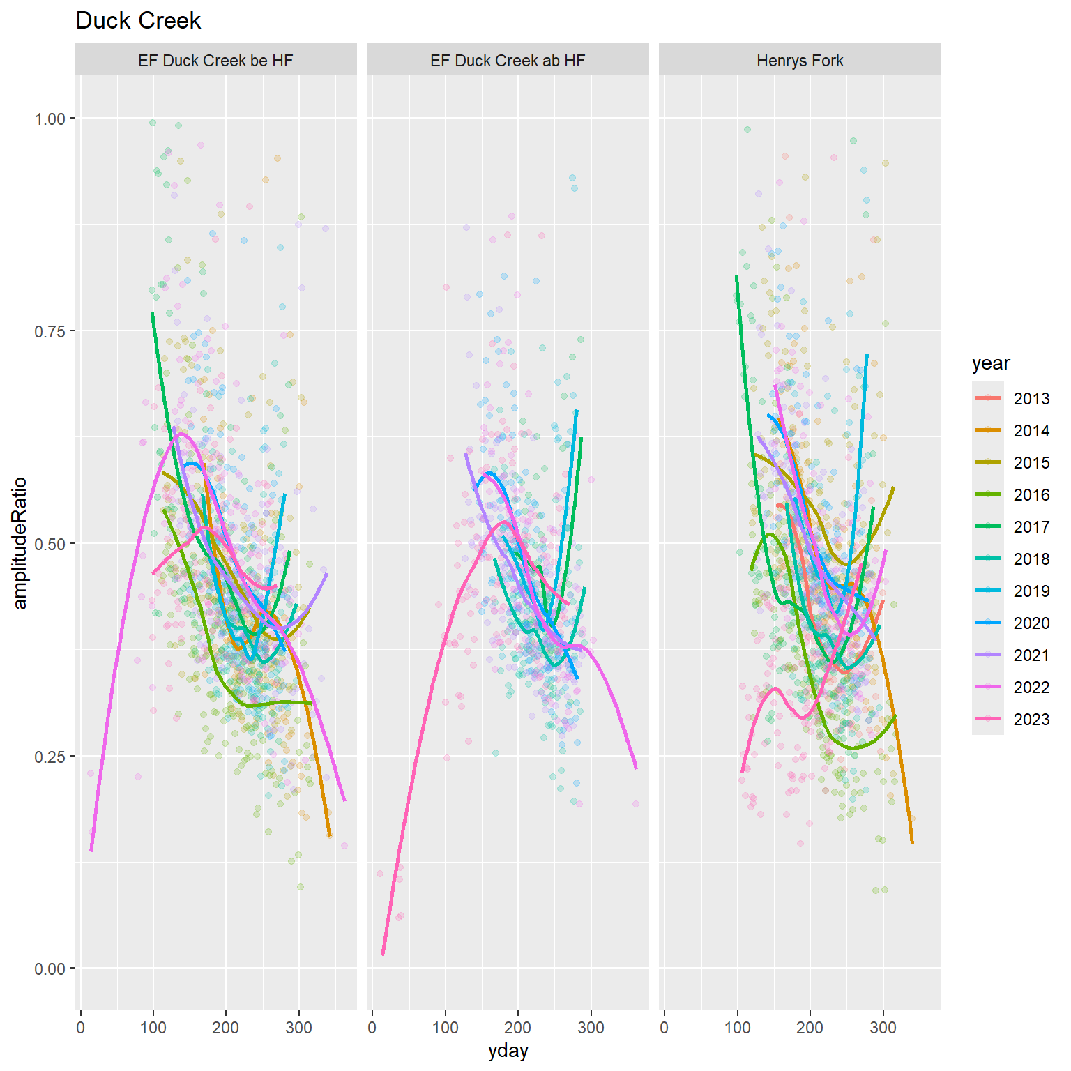
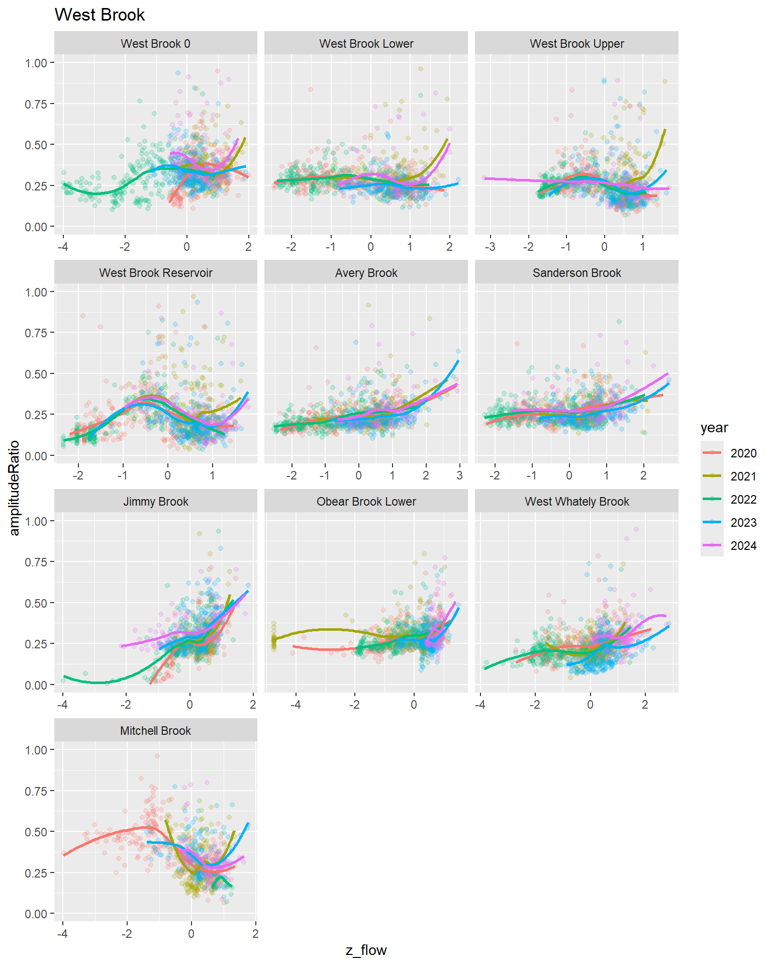
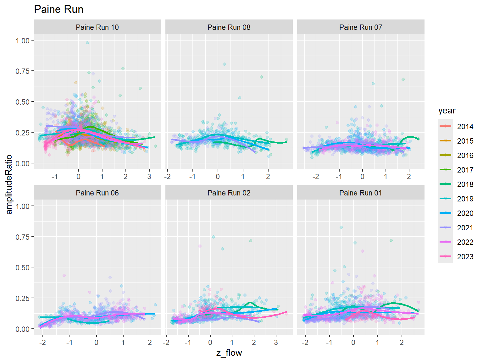
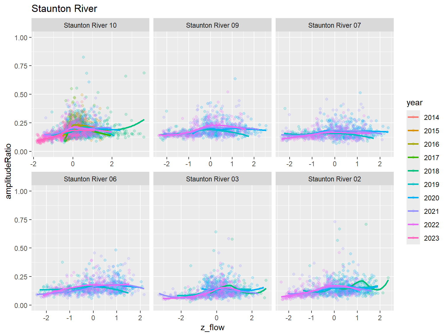
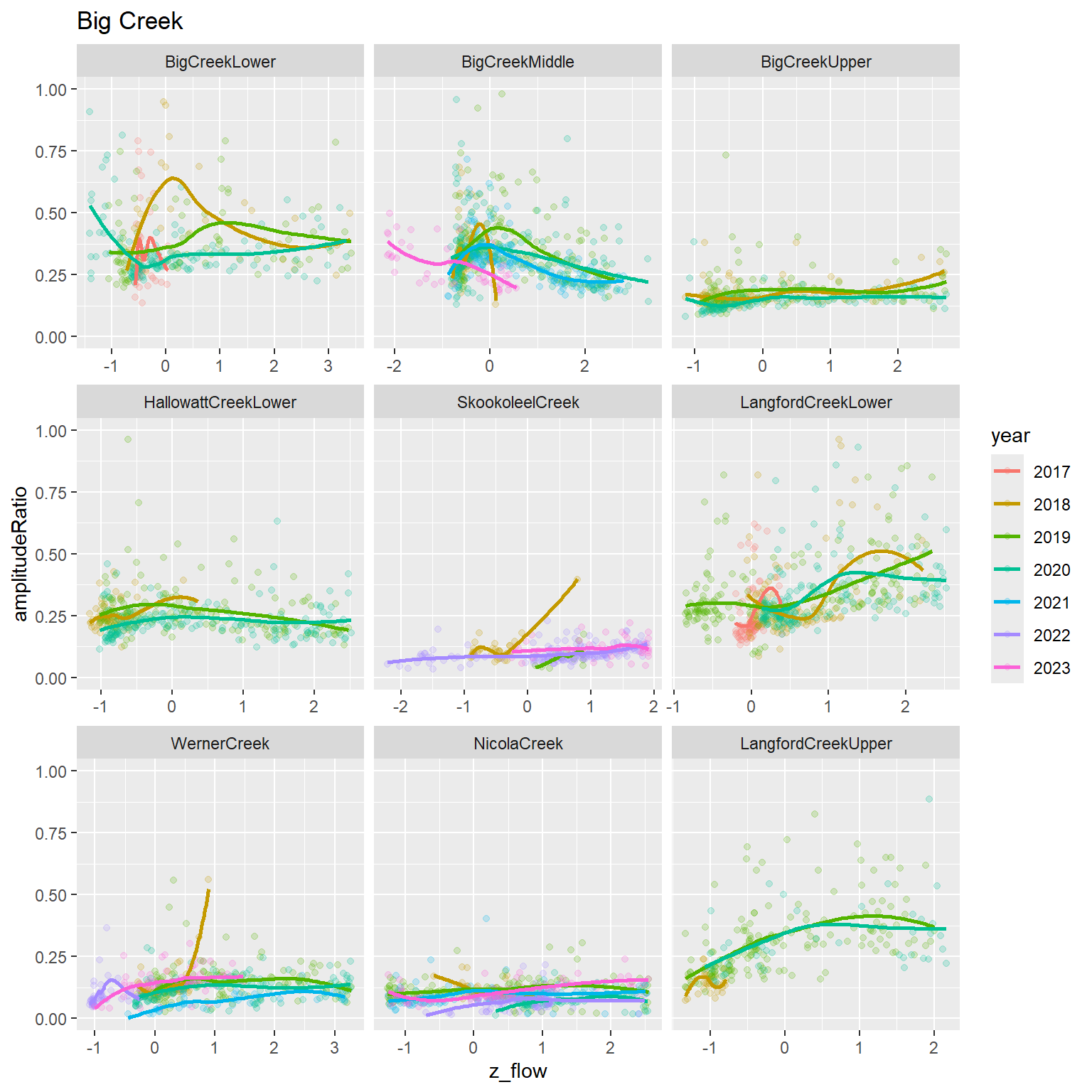
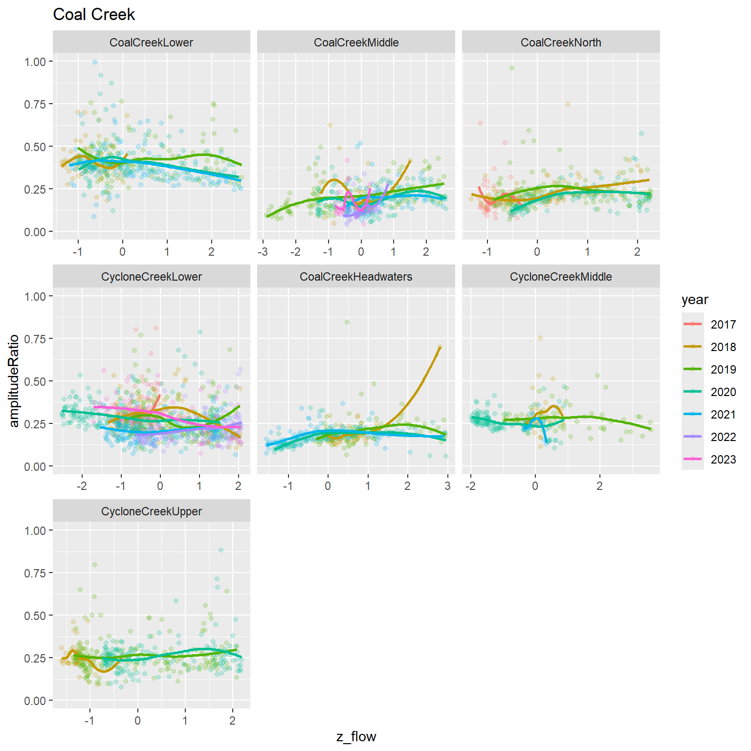
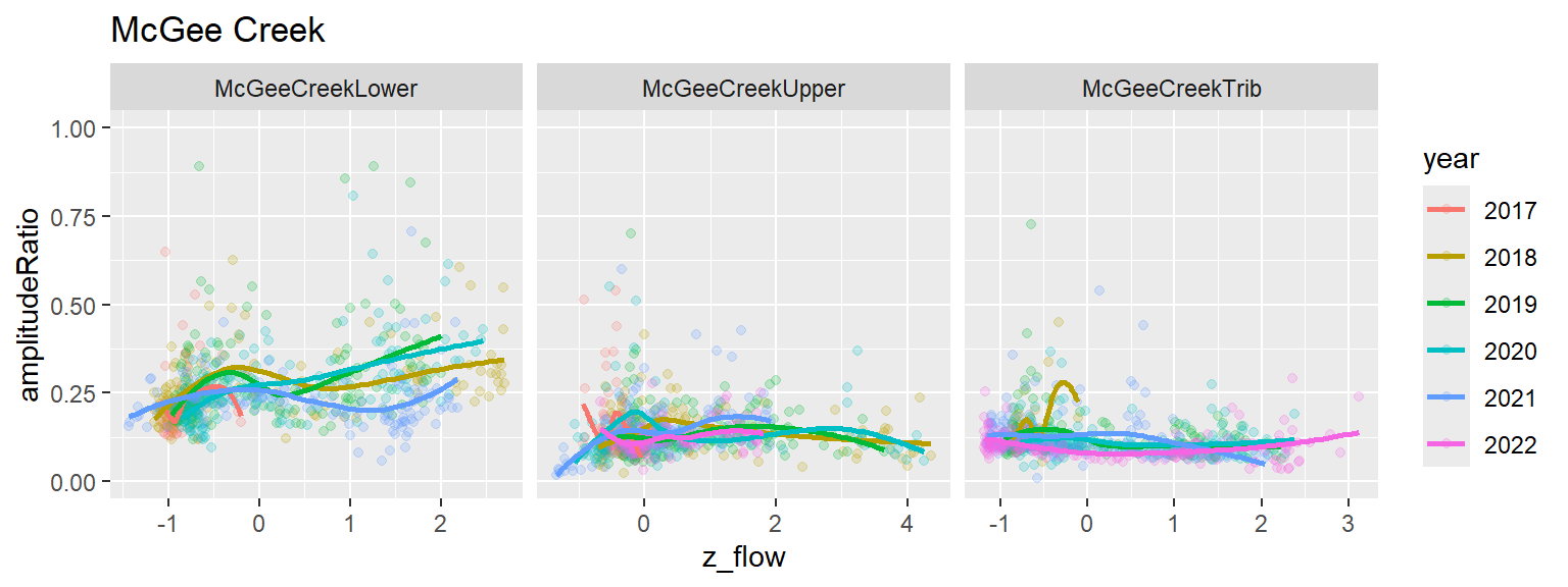
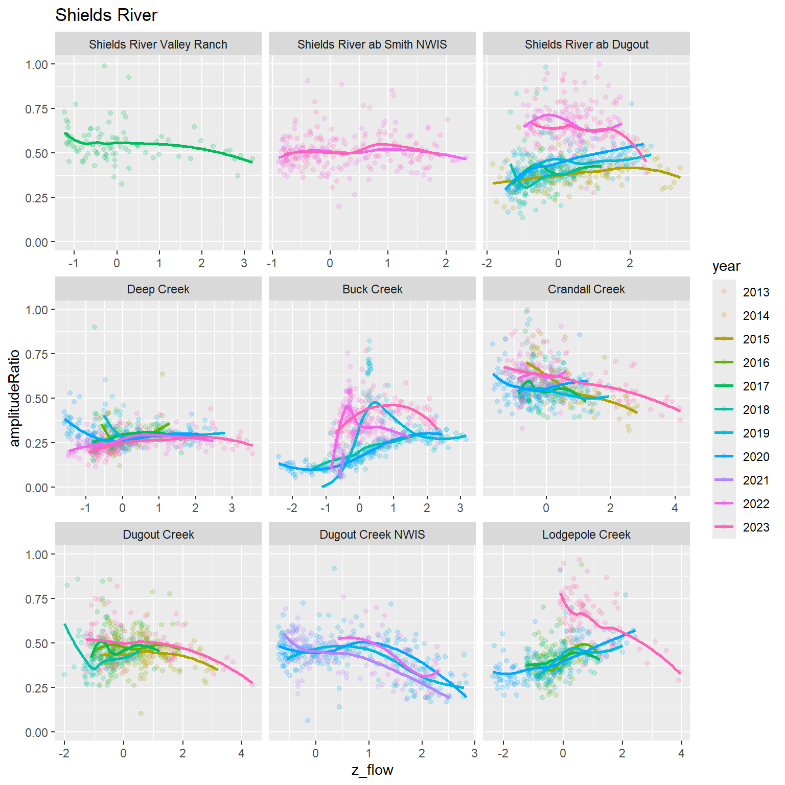
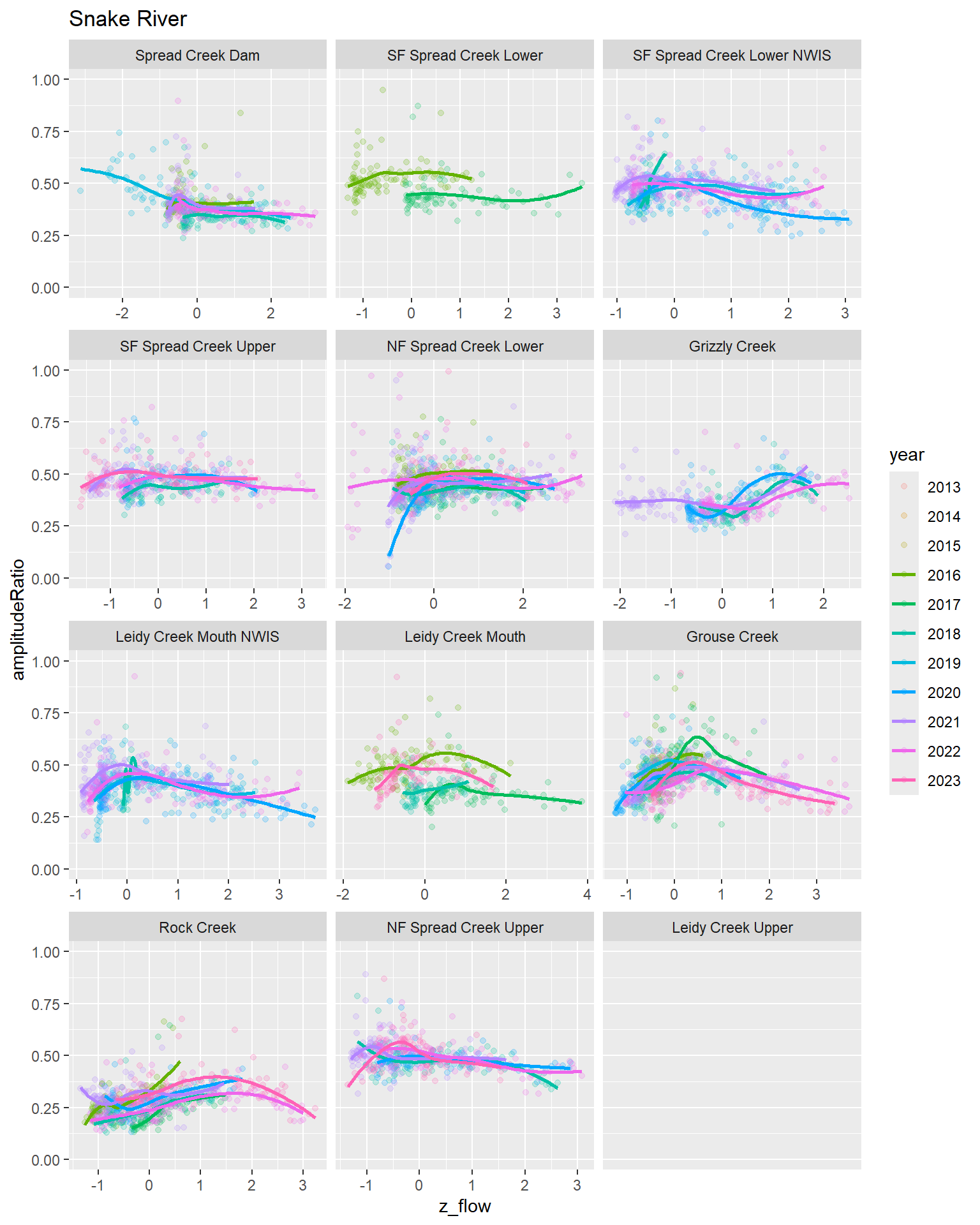
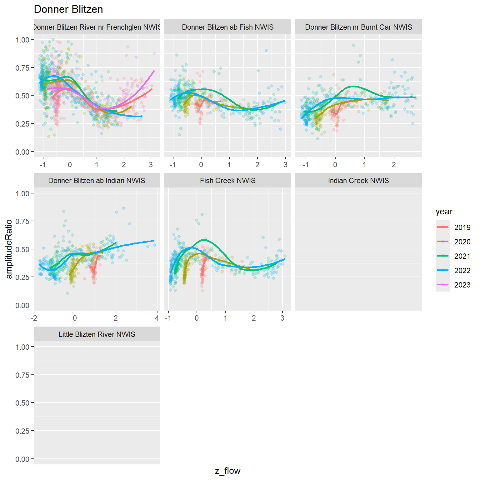
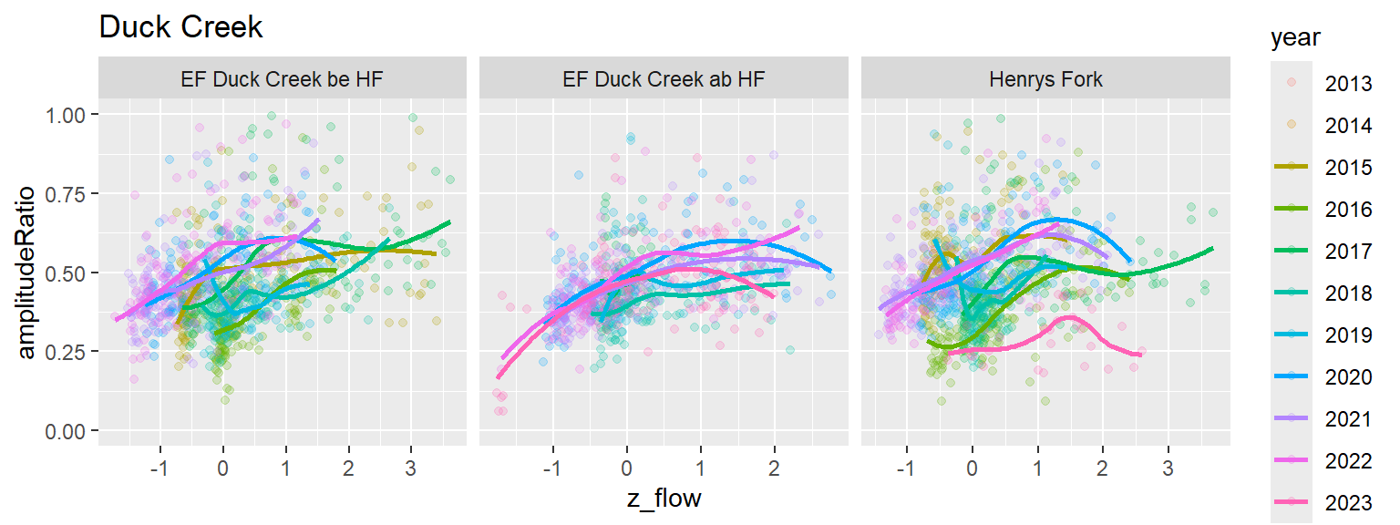
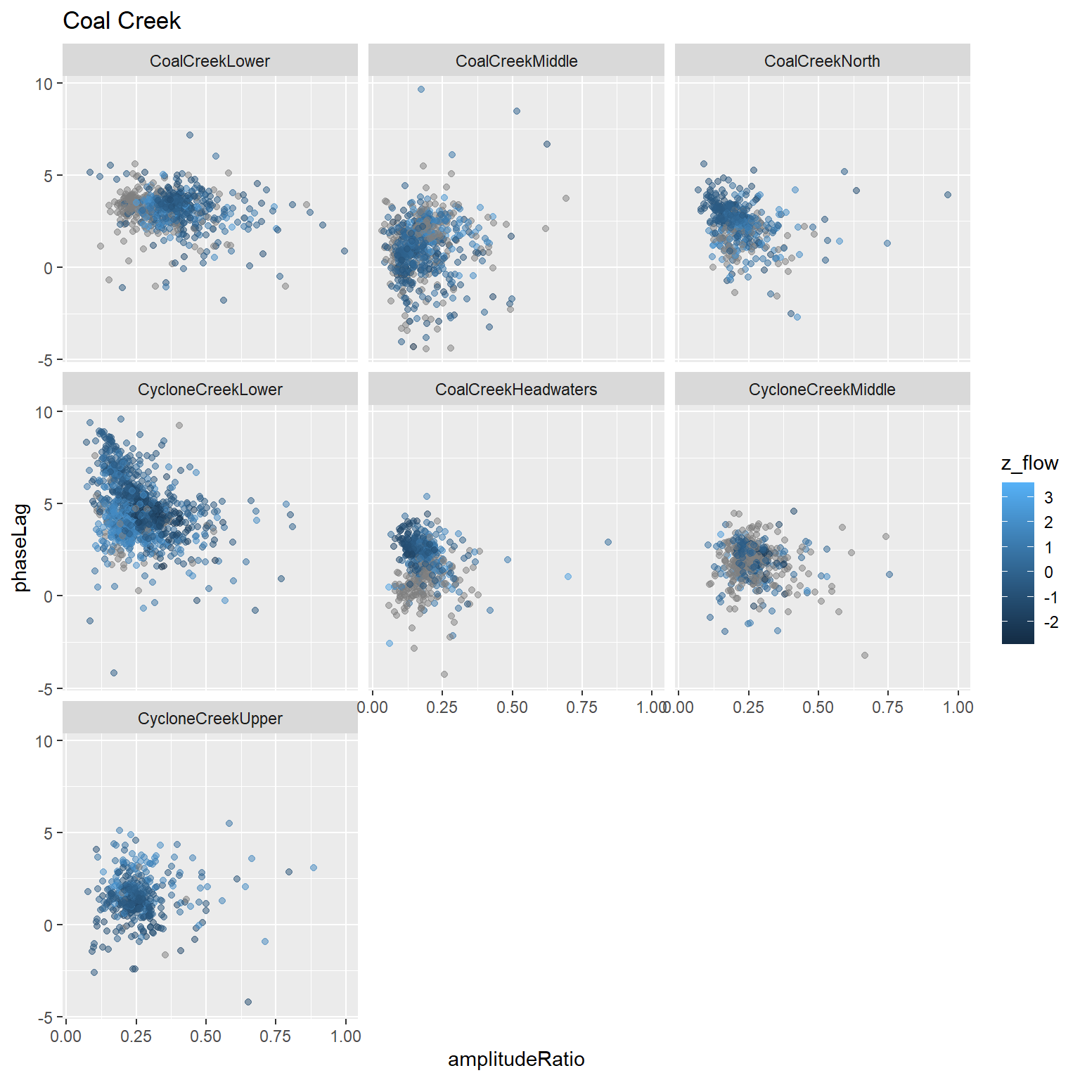
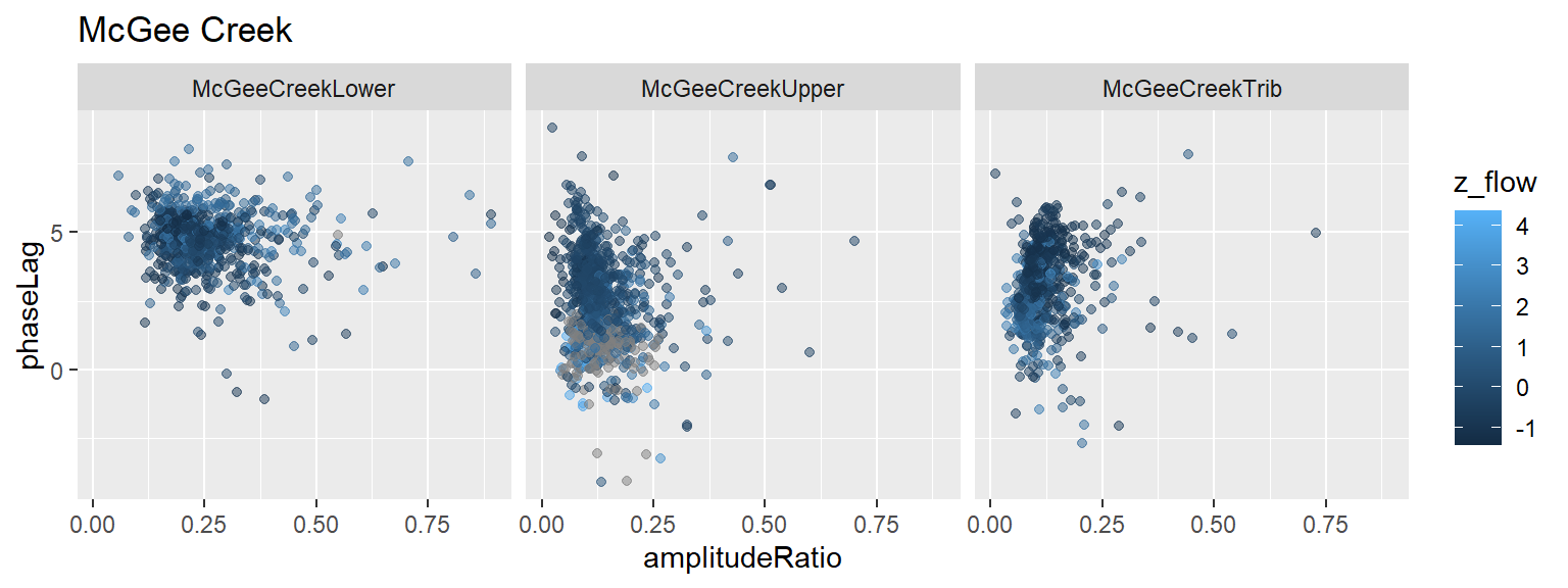
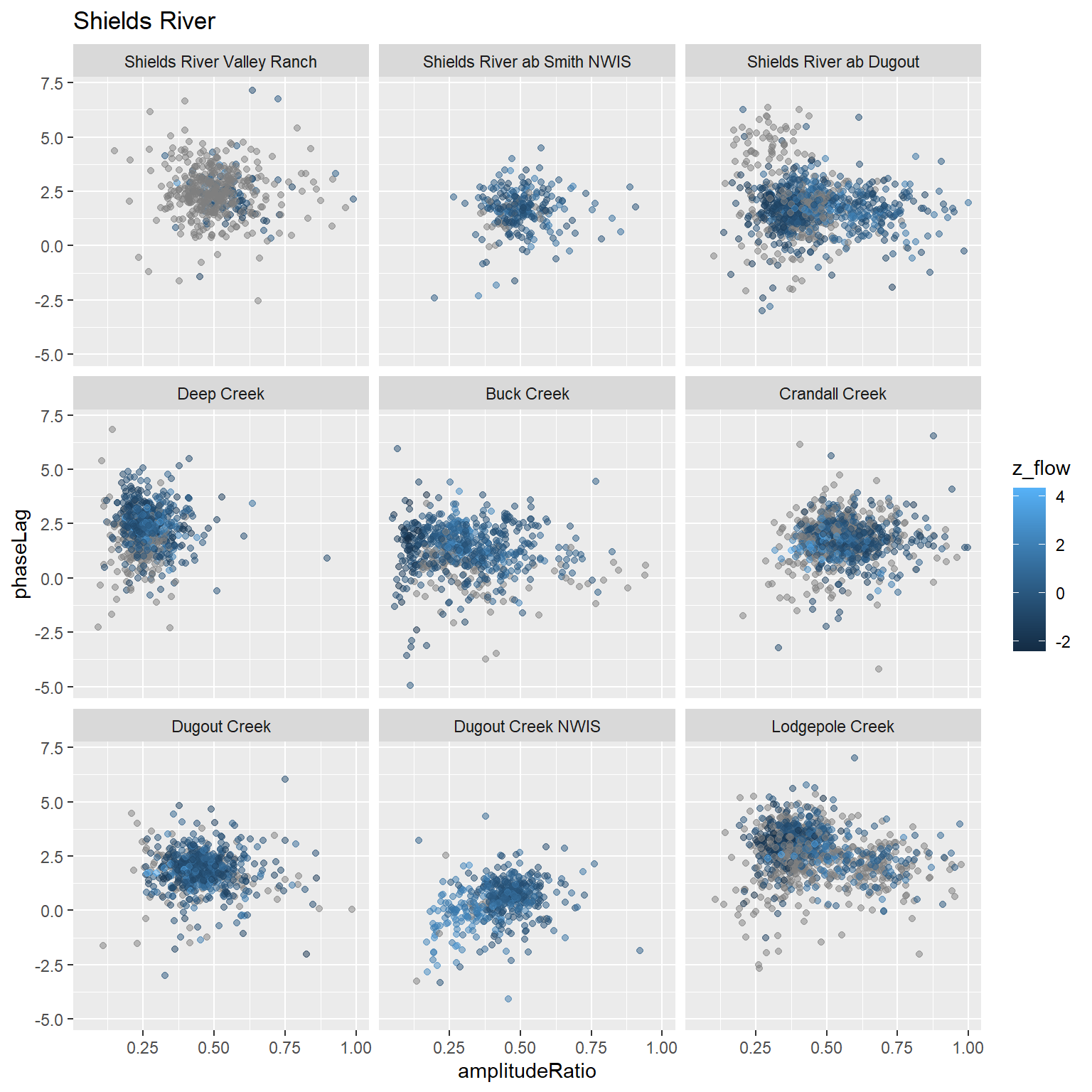
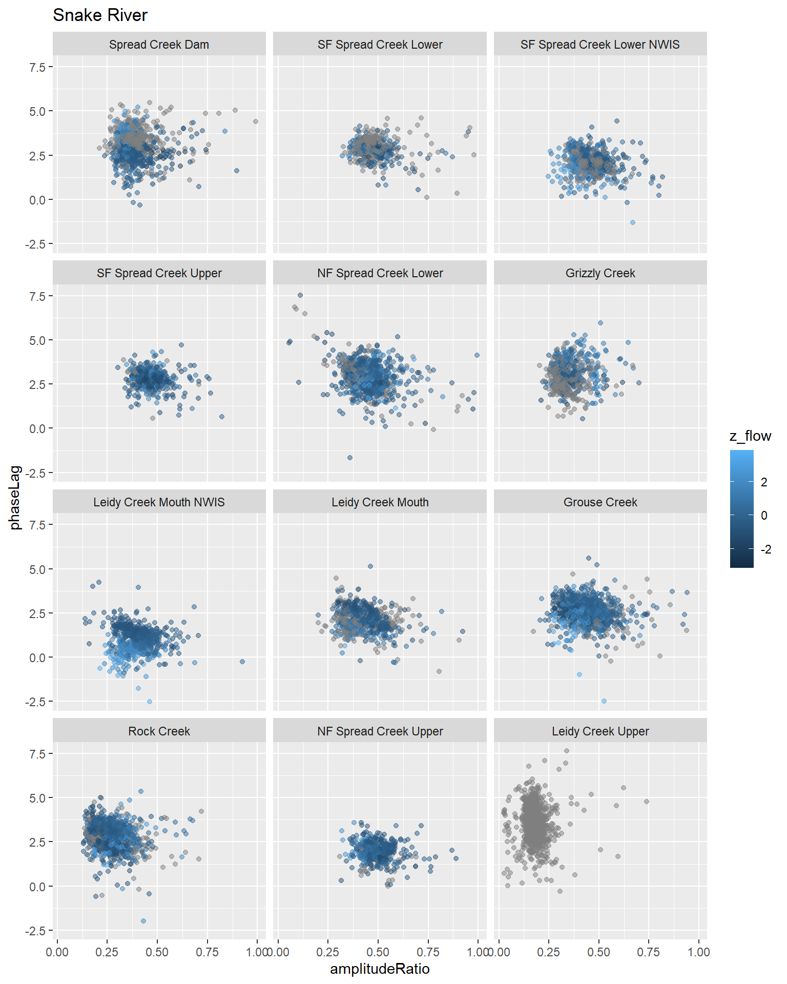
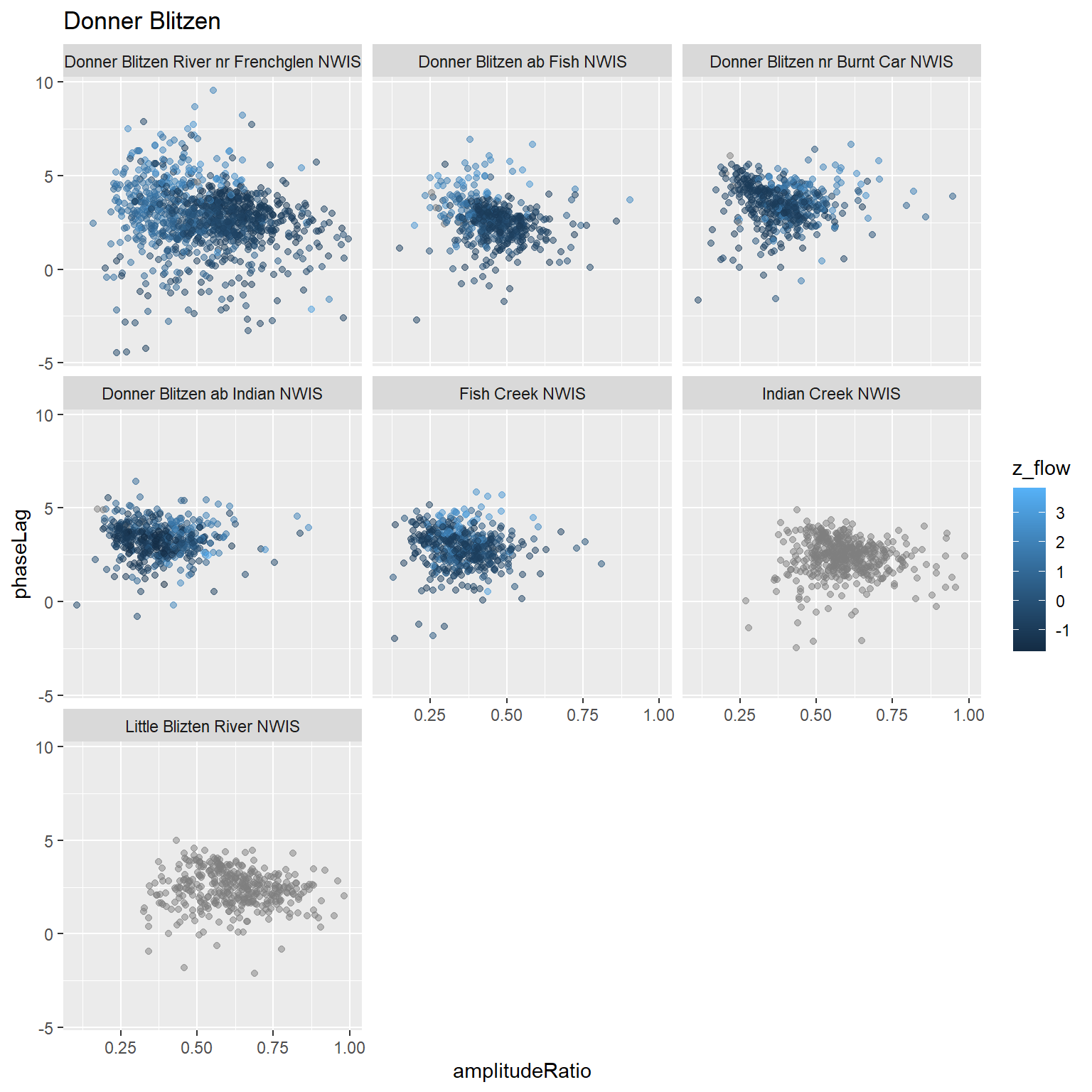
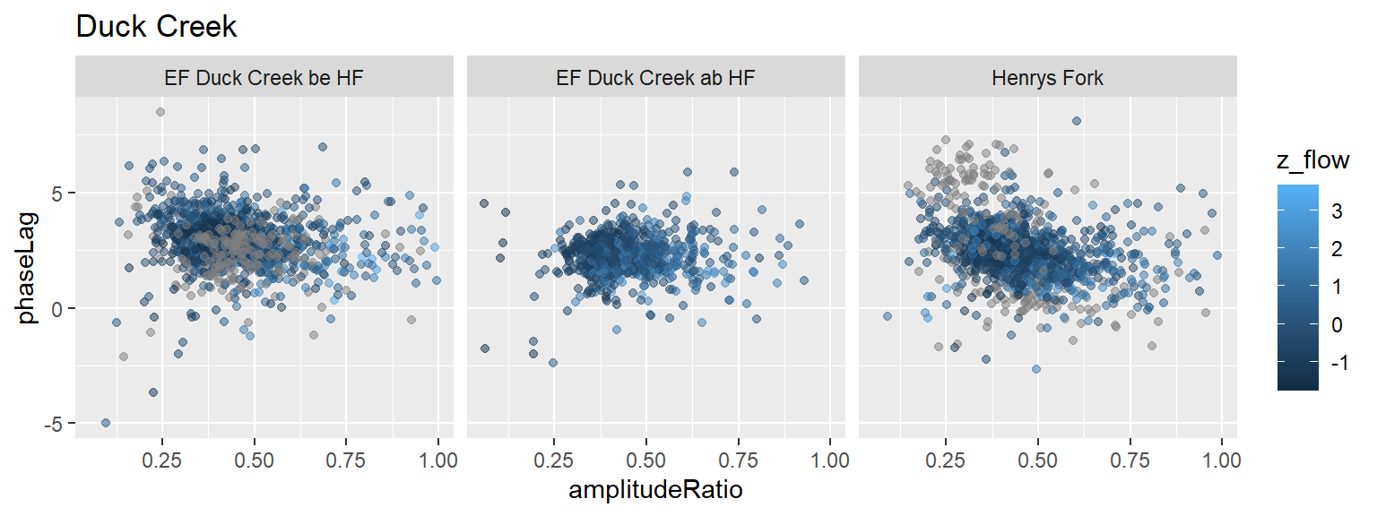
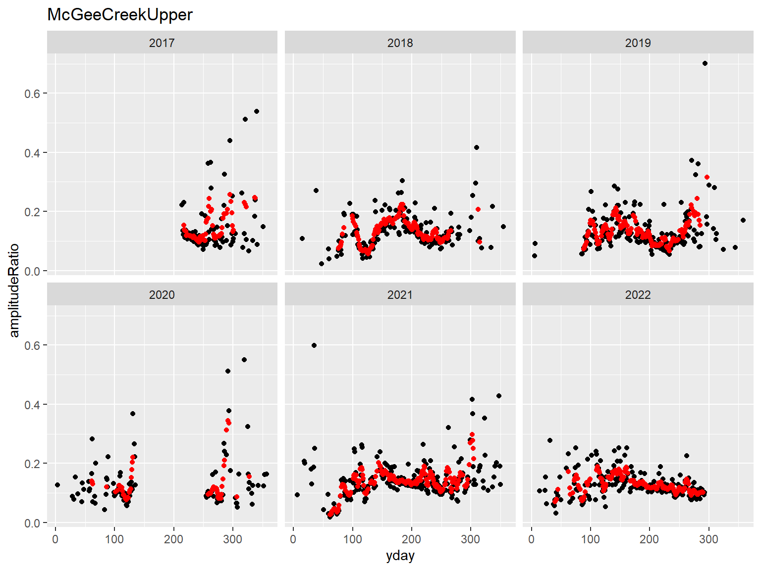
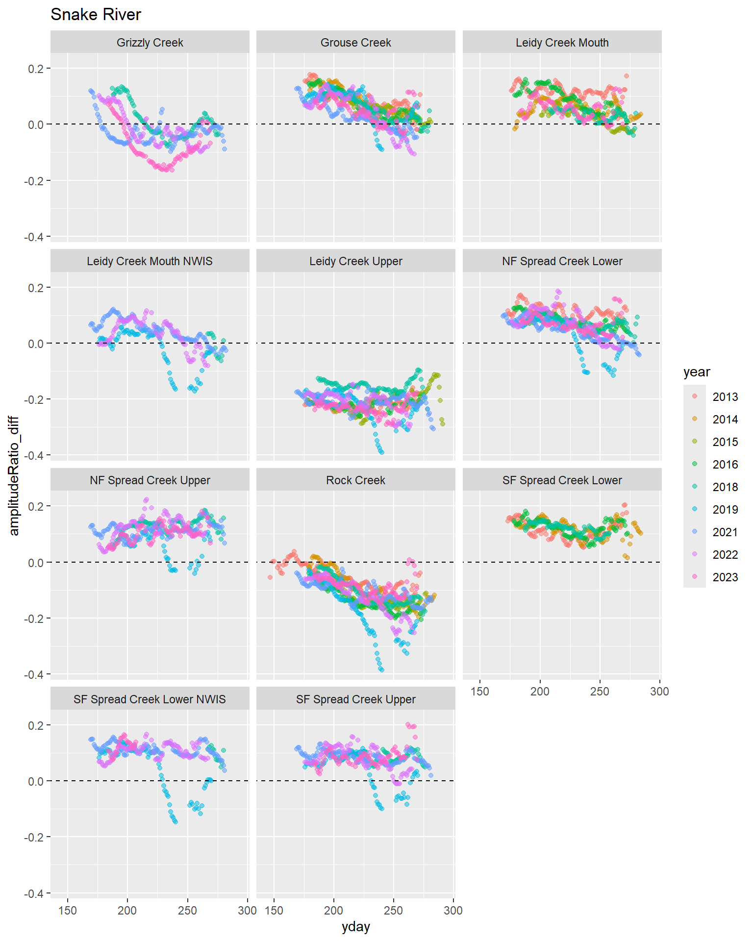
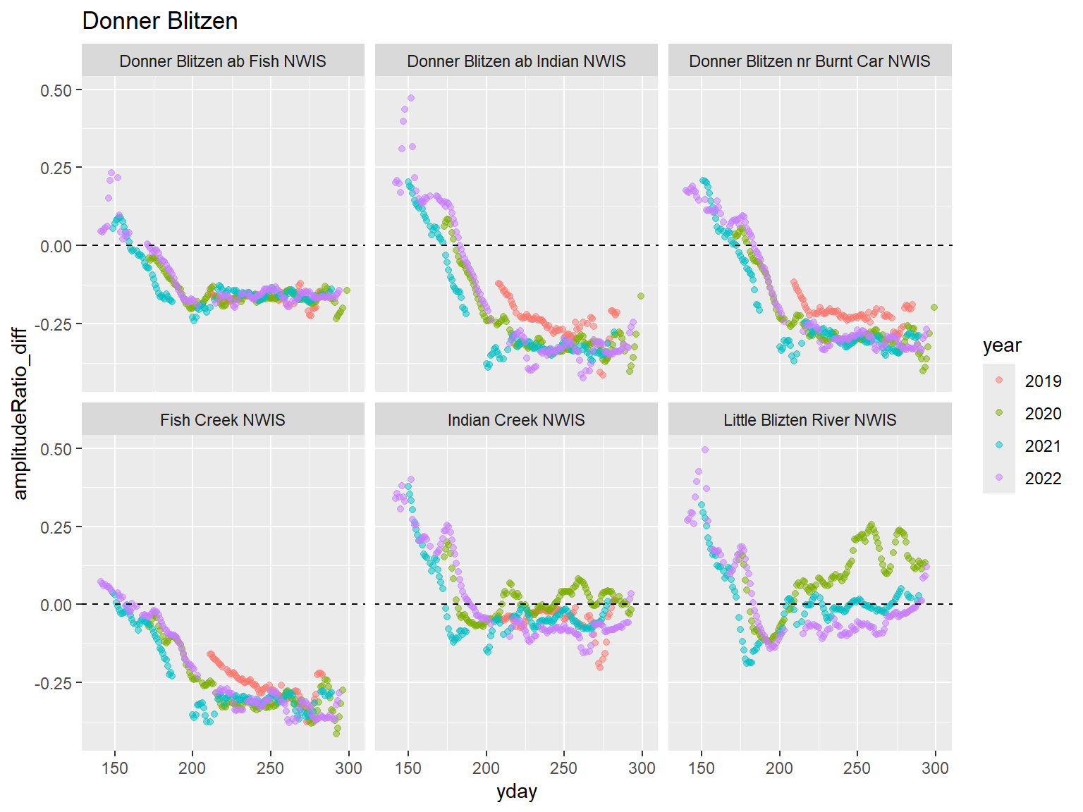
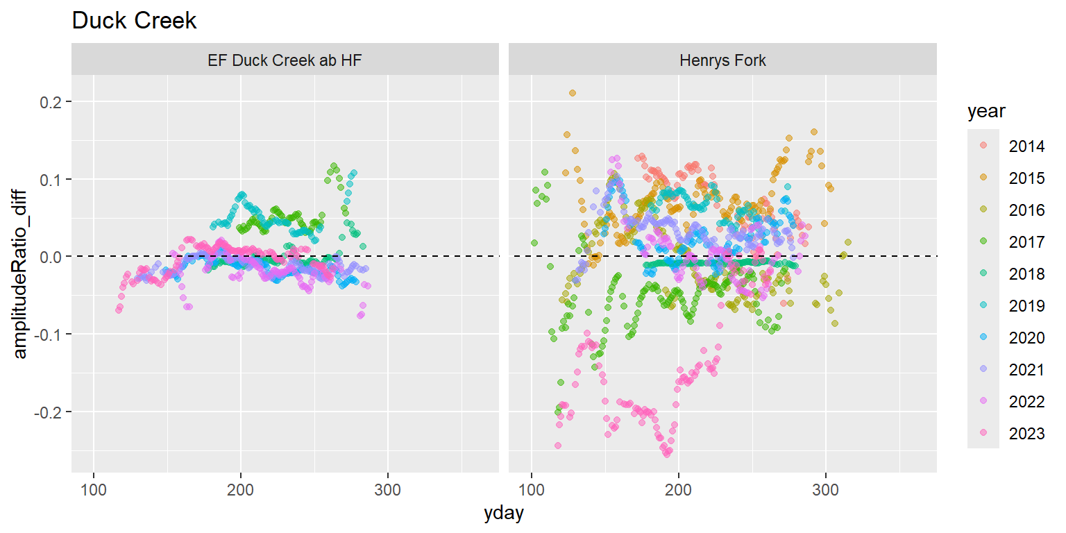
Amplitude ratio: amplitude_water - amplitude_air. Generally, lower amplitude ratios (greater decoupling between air and water temperature sinusoids) are indicative of greater fractional groundwater inputs. (In Rey et al. 2024, Ar values tend to be most similar among tributary/mainstem sites during periods of high surface water input. I.e., high flows homogenize spatial variation in groundwater-surface water dynamics).

pasta_derived %>% filter(site_name == focal_site, rSquared_air >= 0.7 & rSquared_water >= 0.7) %>% select(date, amplitudeRatio) %>% dygraph(main = focal_site) %>% dyRangeSelector() %>% dyAxis("y", label = "Amplitude ratio") %>% dyOptions(drawPoints = T, strokeWidth = 0, pointSize = 3) %>% dyHighlight(highlightCircleSize = 5)

pasta_derived %>% filter(site_name == focal_site, rSquared_air >= 0.7 & rSquared_water >= 0.7) %>% ggplot(aes(x = yday, y = amplitudeRatio, color = z_flow)) + geom_point() + ggtitle(focal_site) + geom_smooth(method = "lm", formula = y ~ poly(x, 2)) + facet_wrap(~year)

pasta_derived %>% filter(site_name == focal_site, rSquared_air >= 0.7 & rSquared_water >= 0.7) %>% ggplot(aes(x = z_flow, y = amplitudeRatio, color = as.factor(year))) + geom_point(alpha= 0.3) + ggtitle(focal_site) + geom_smooth(se = FALSE)

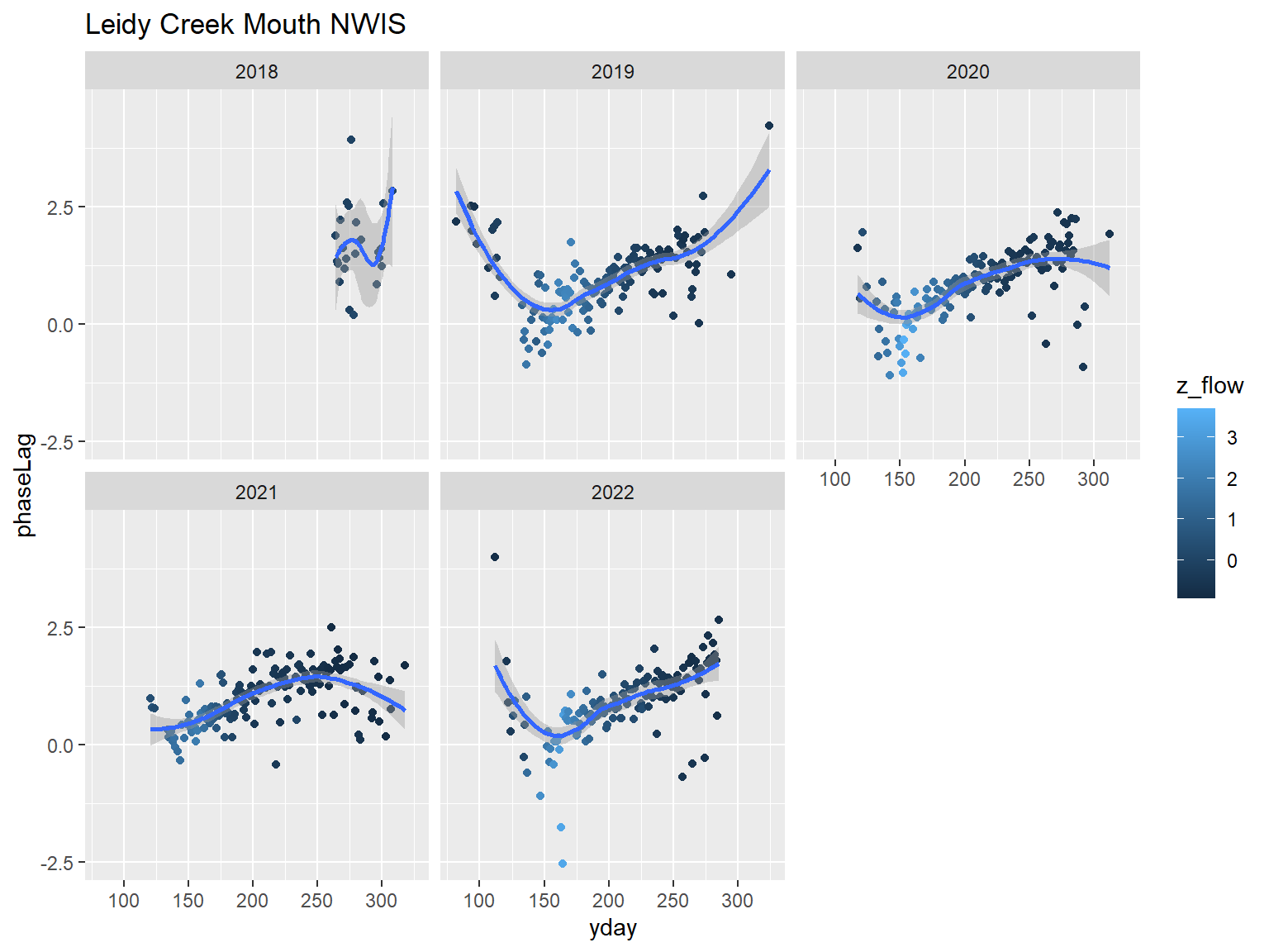
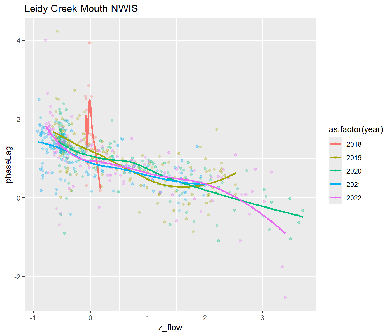
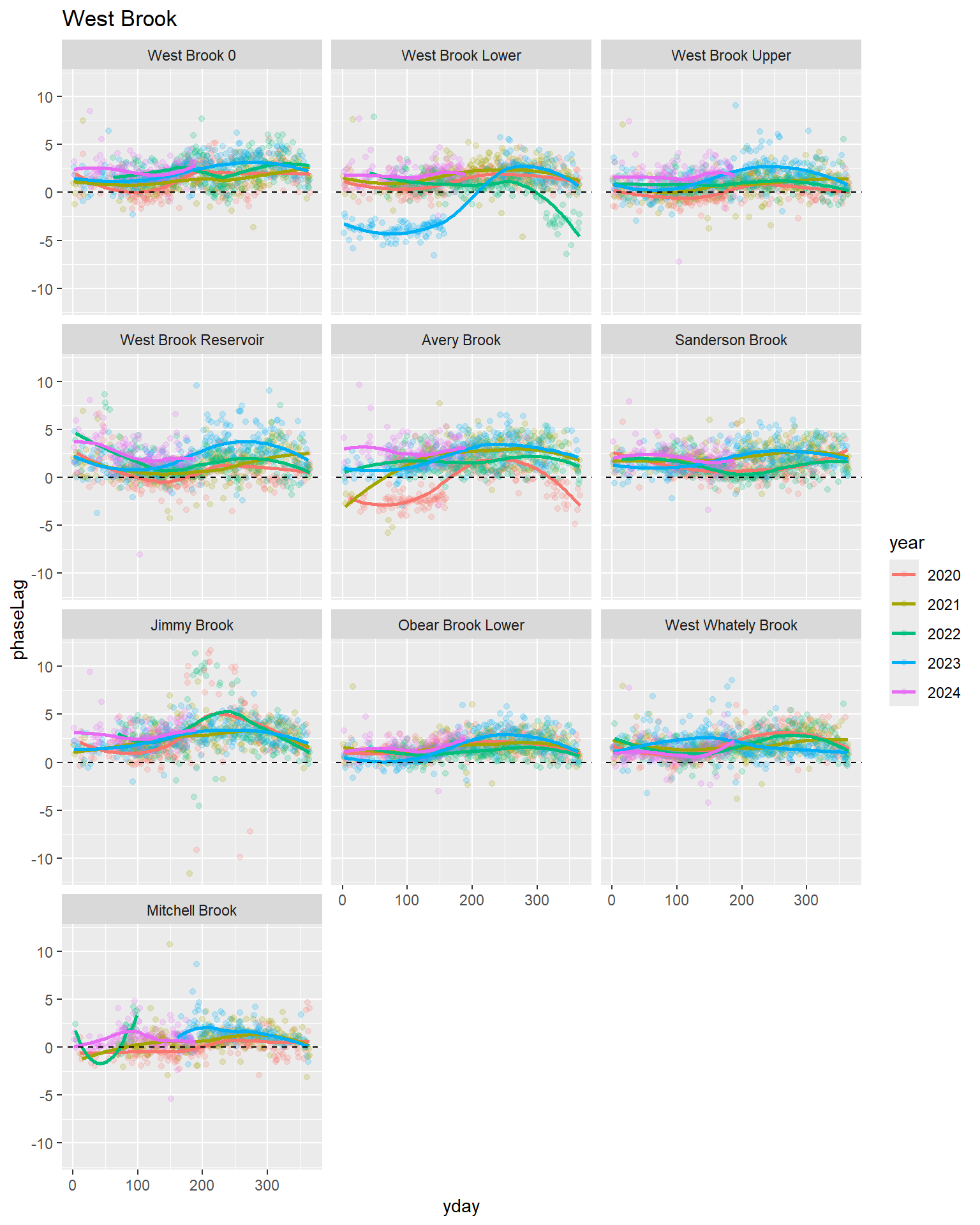
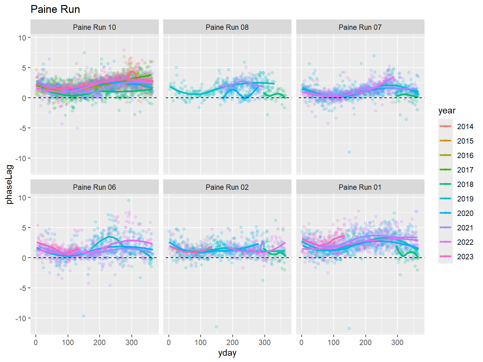
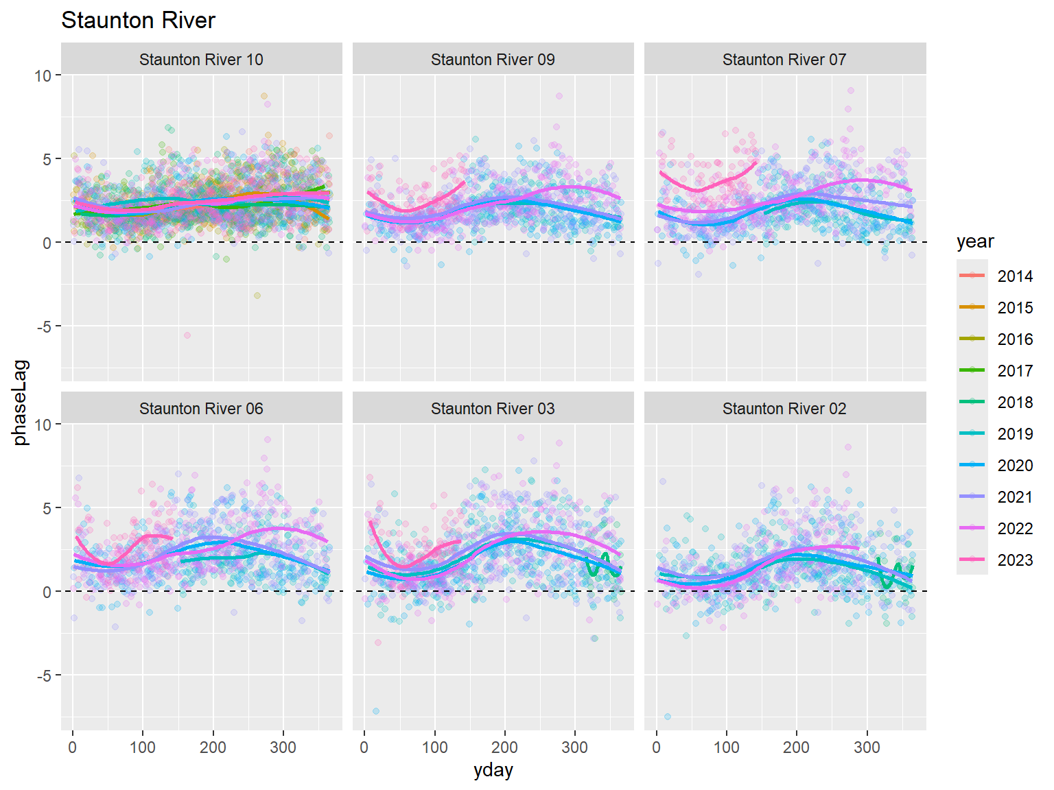
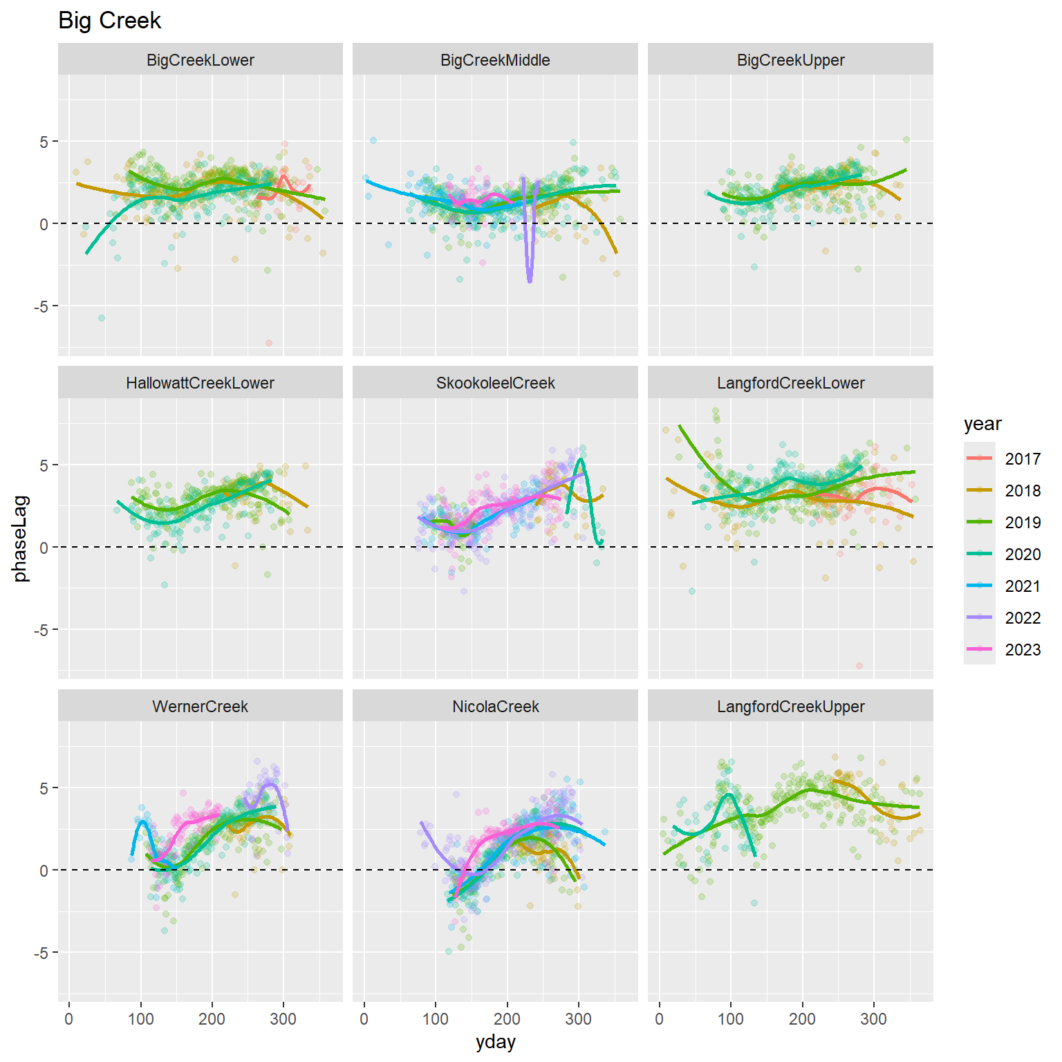
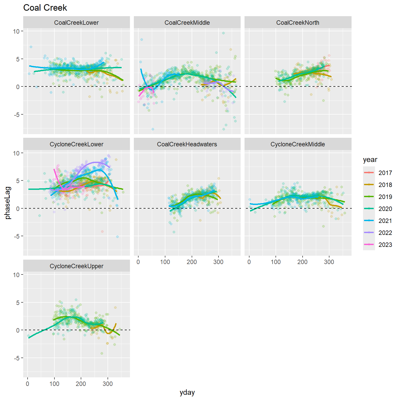
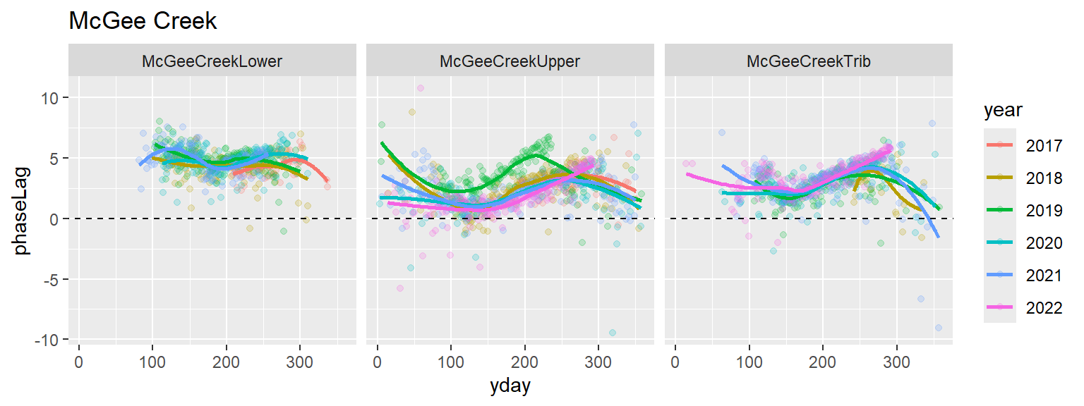
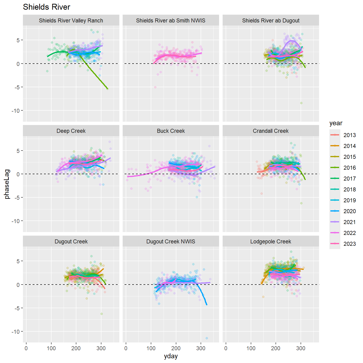
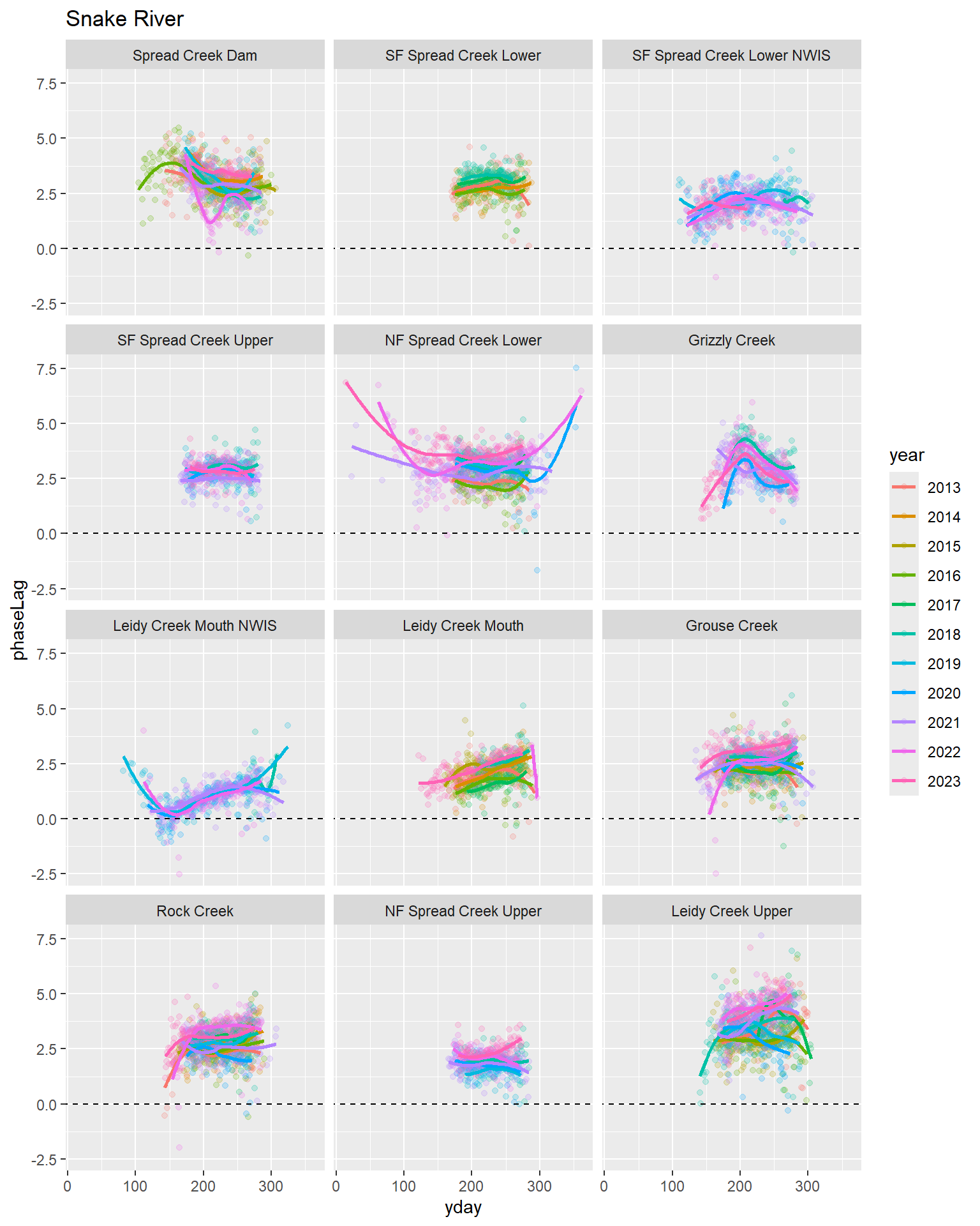
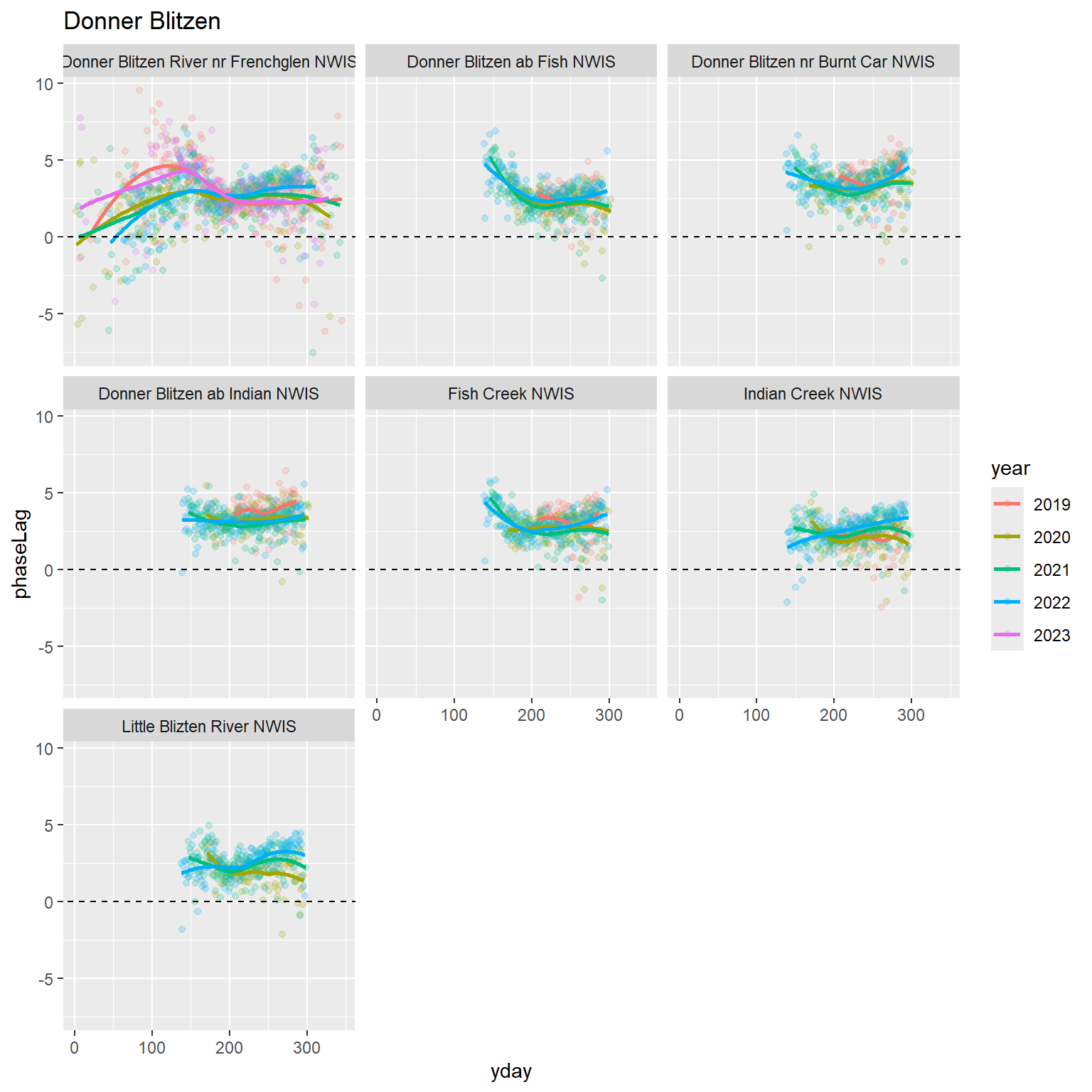
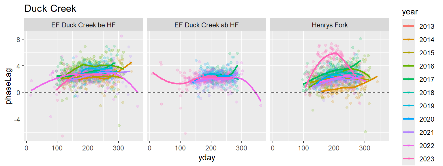
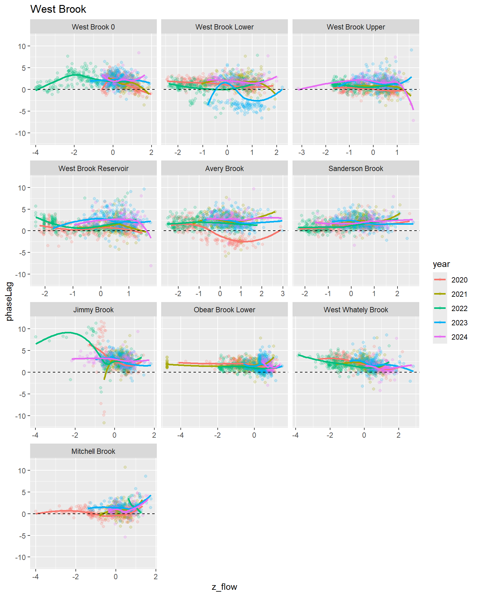
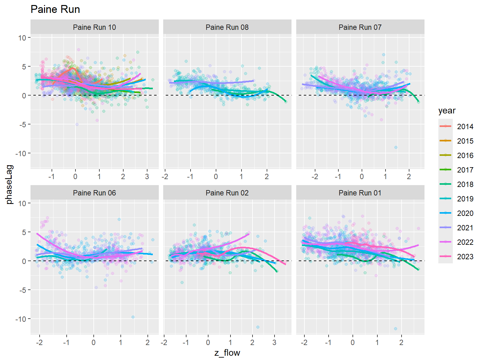
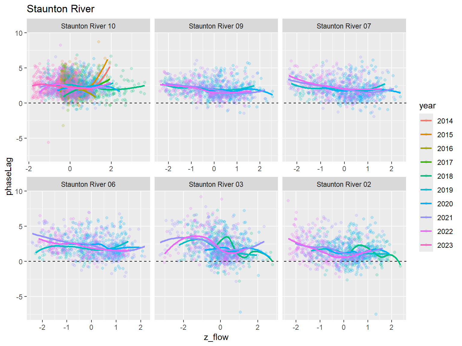
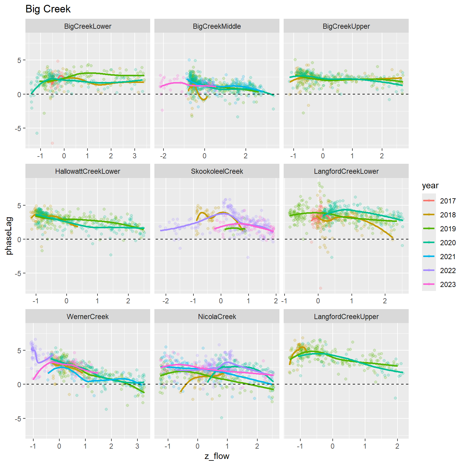
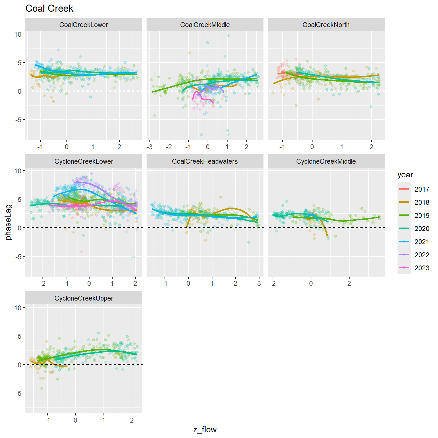
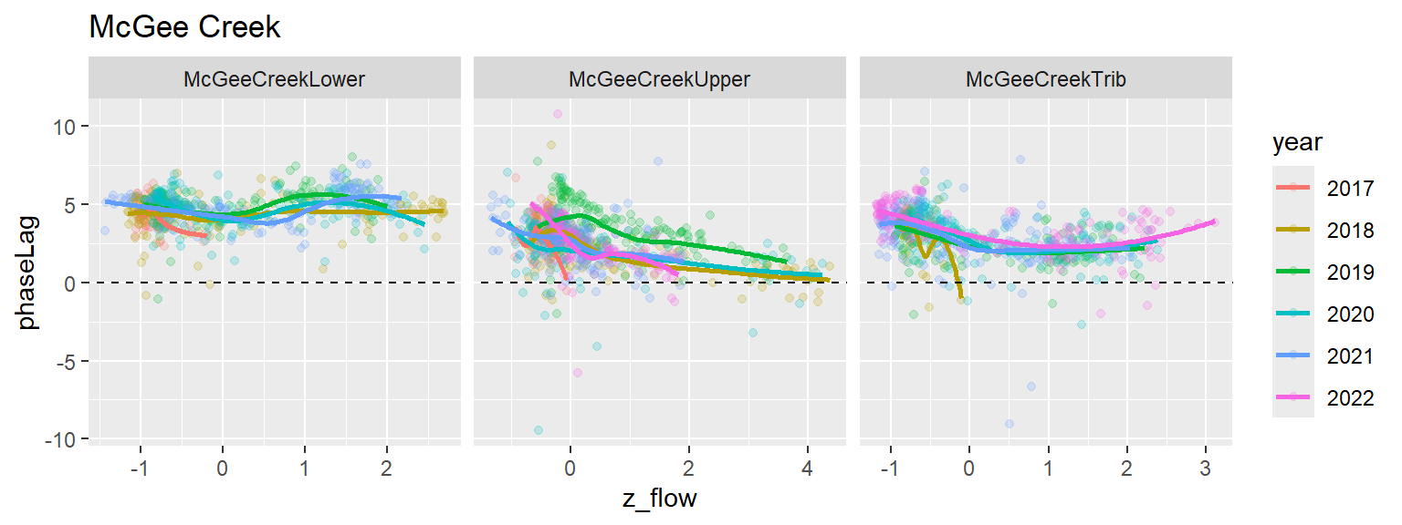
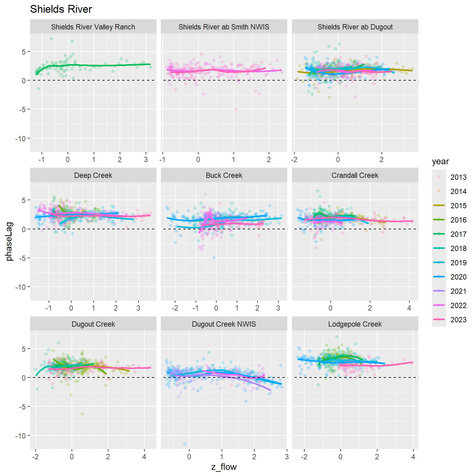
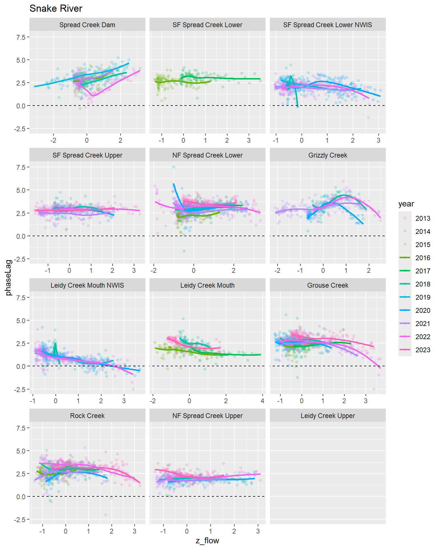
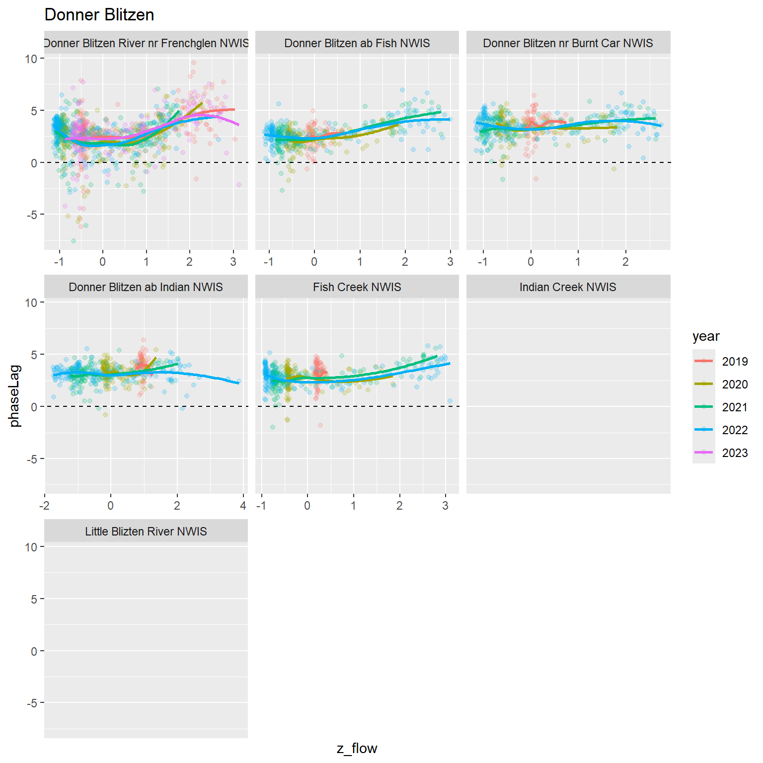
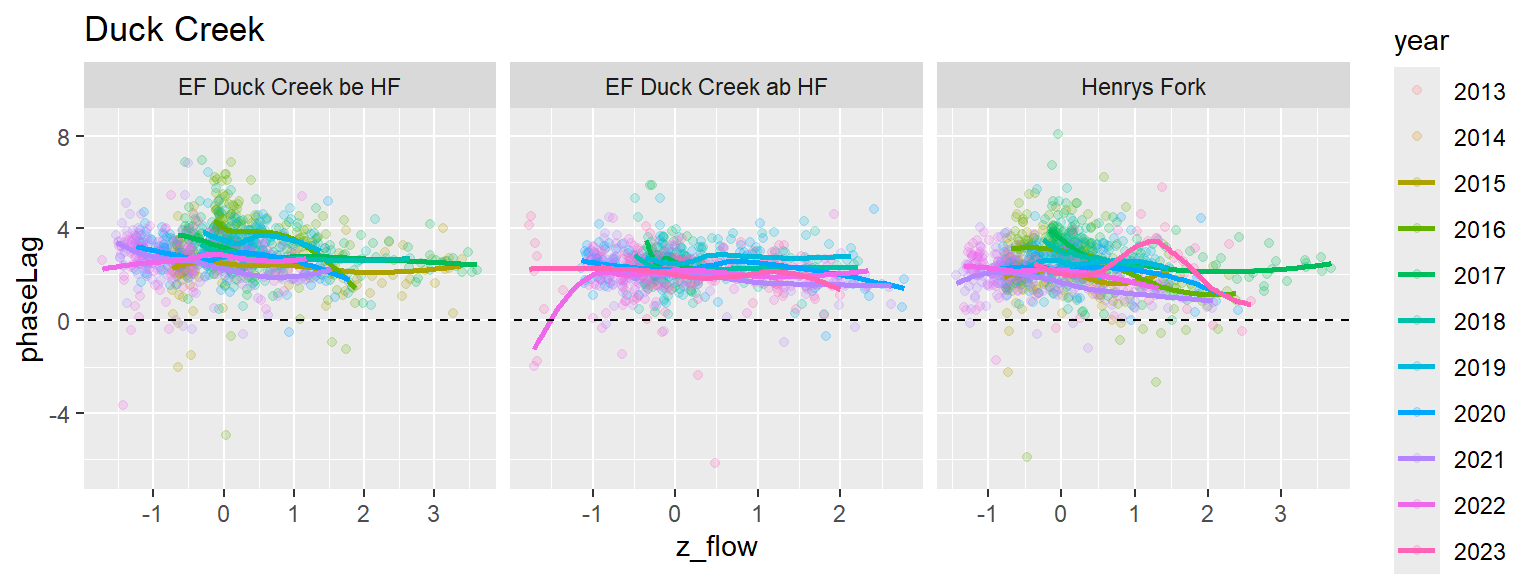
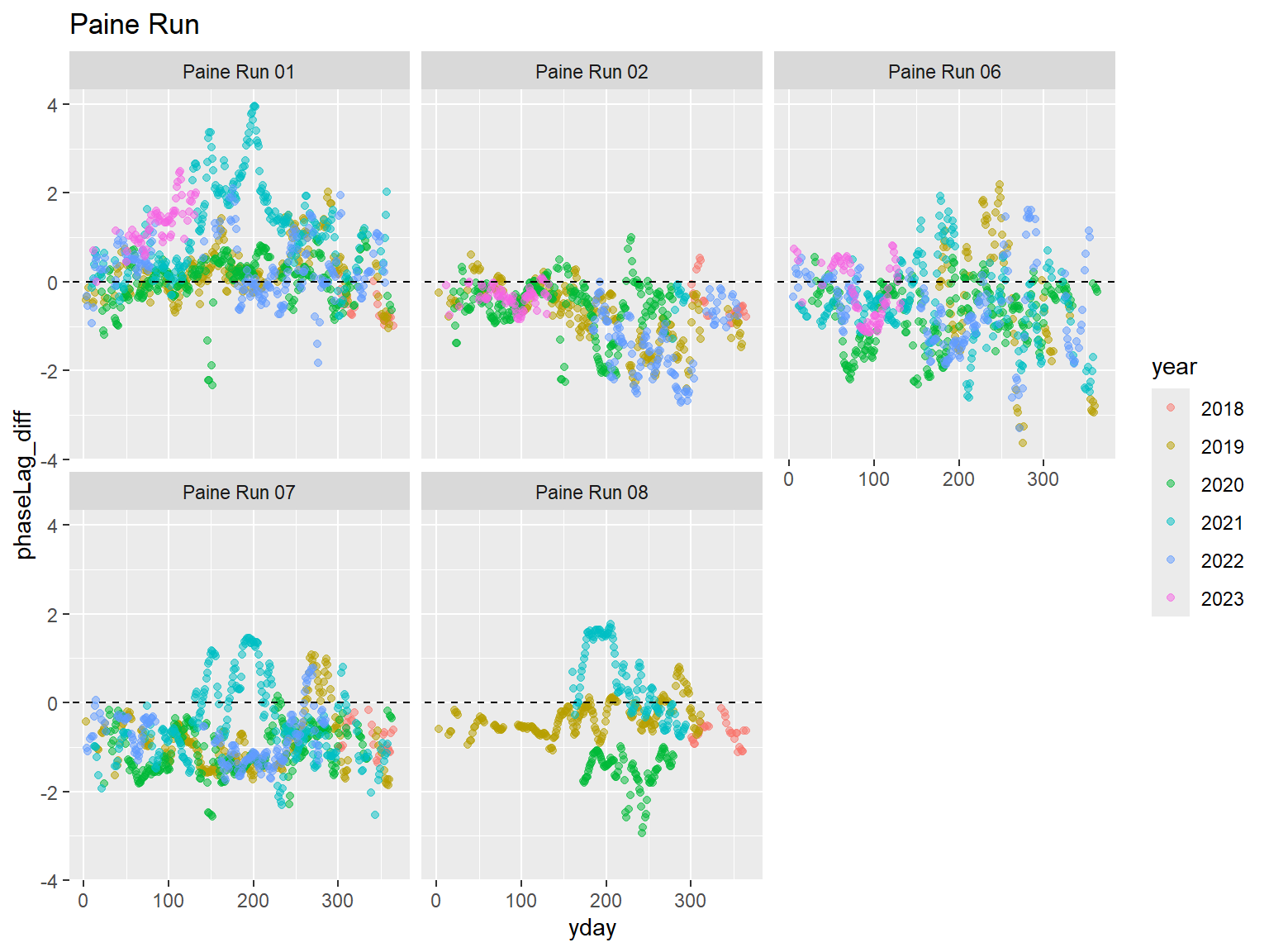
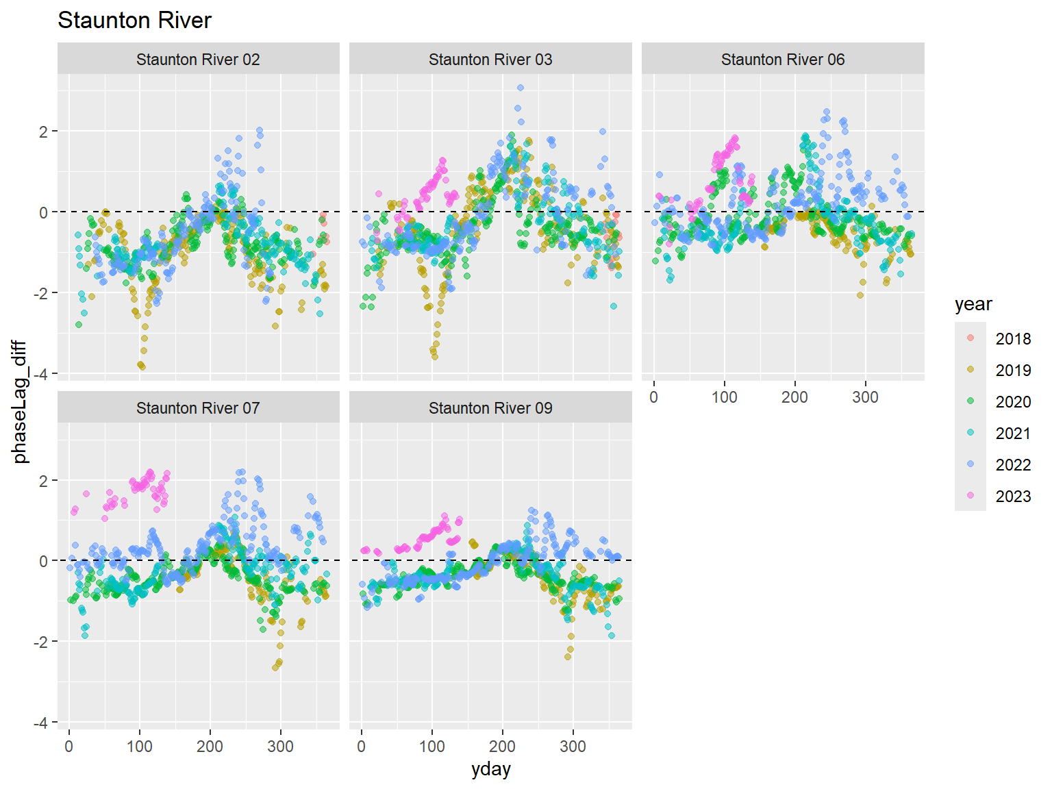
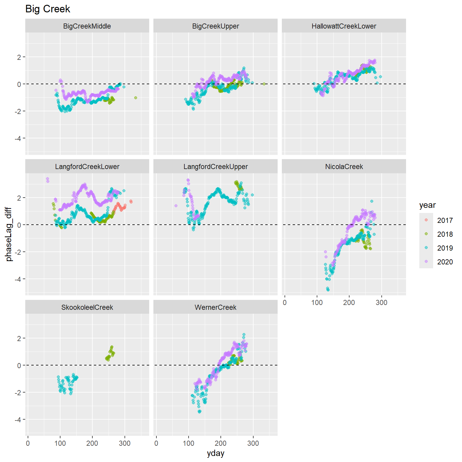
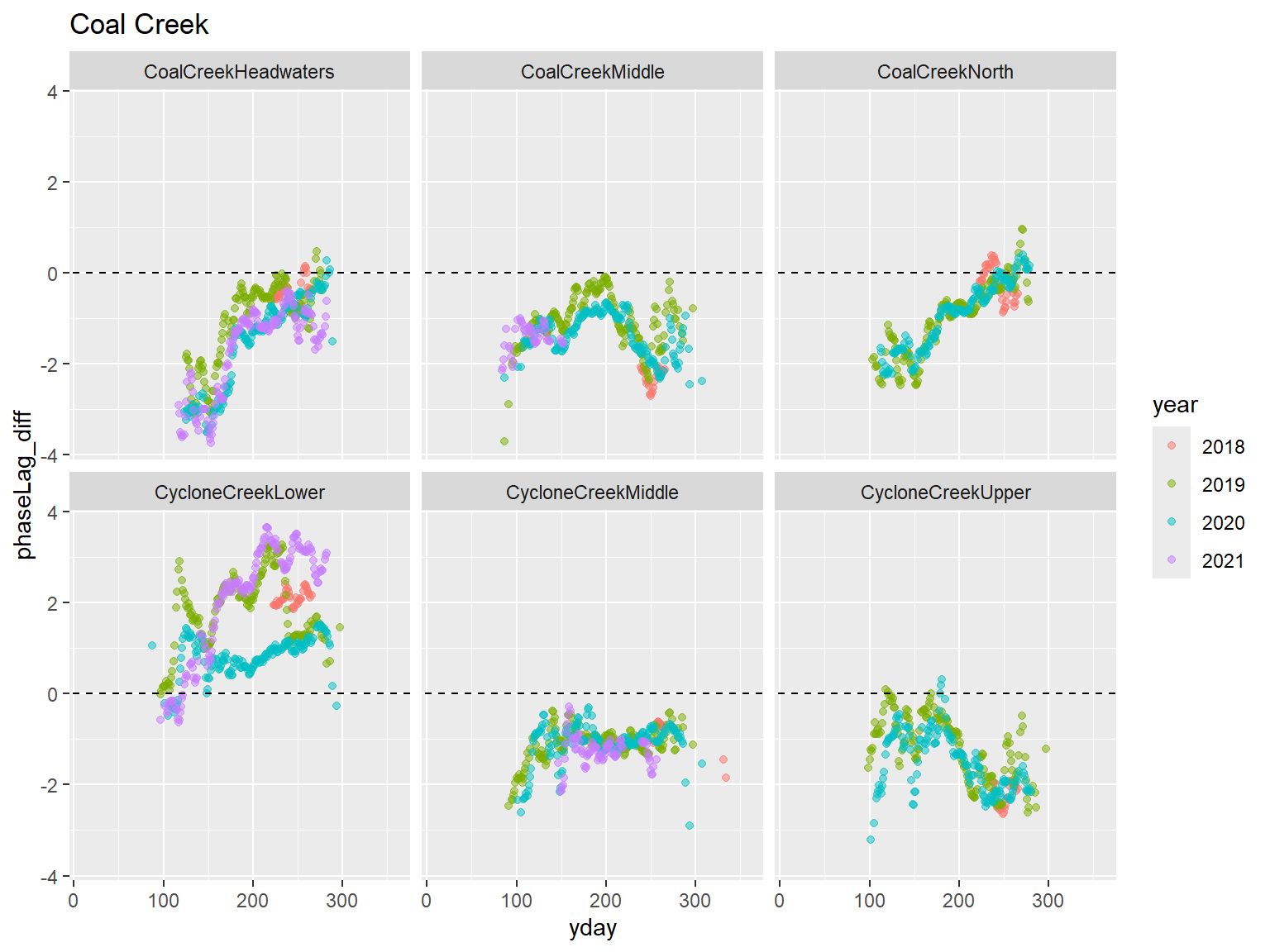
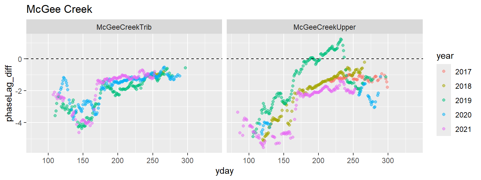
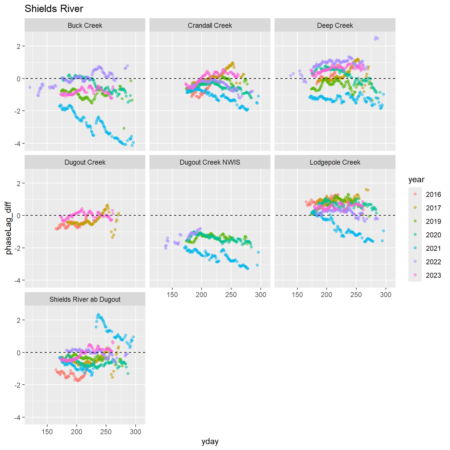
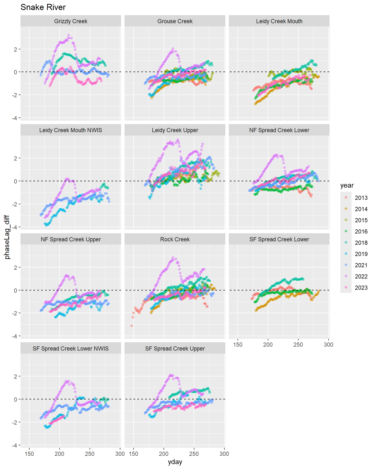
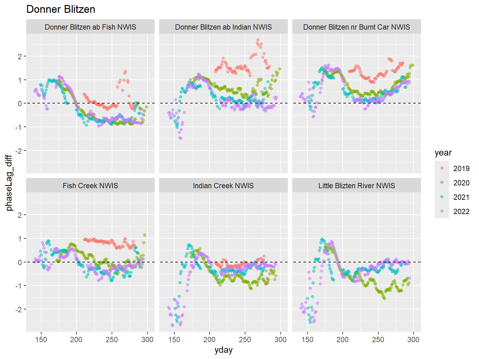
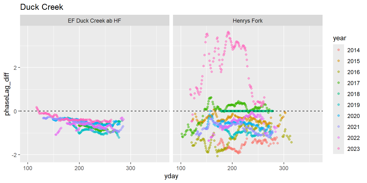
7.4.1.2 Phase lag

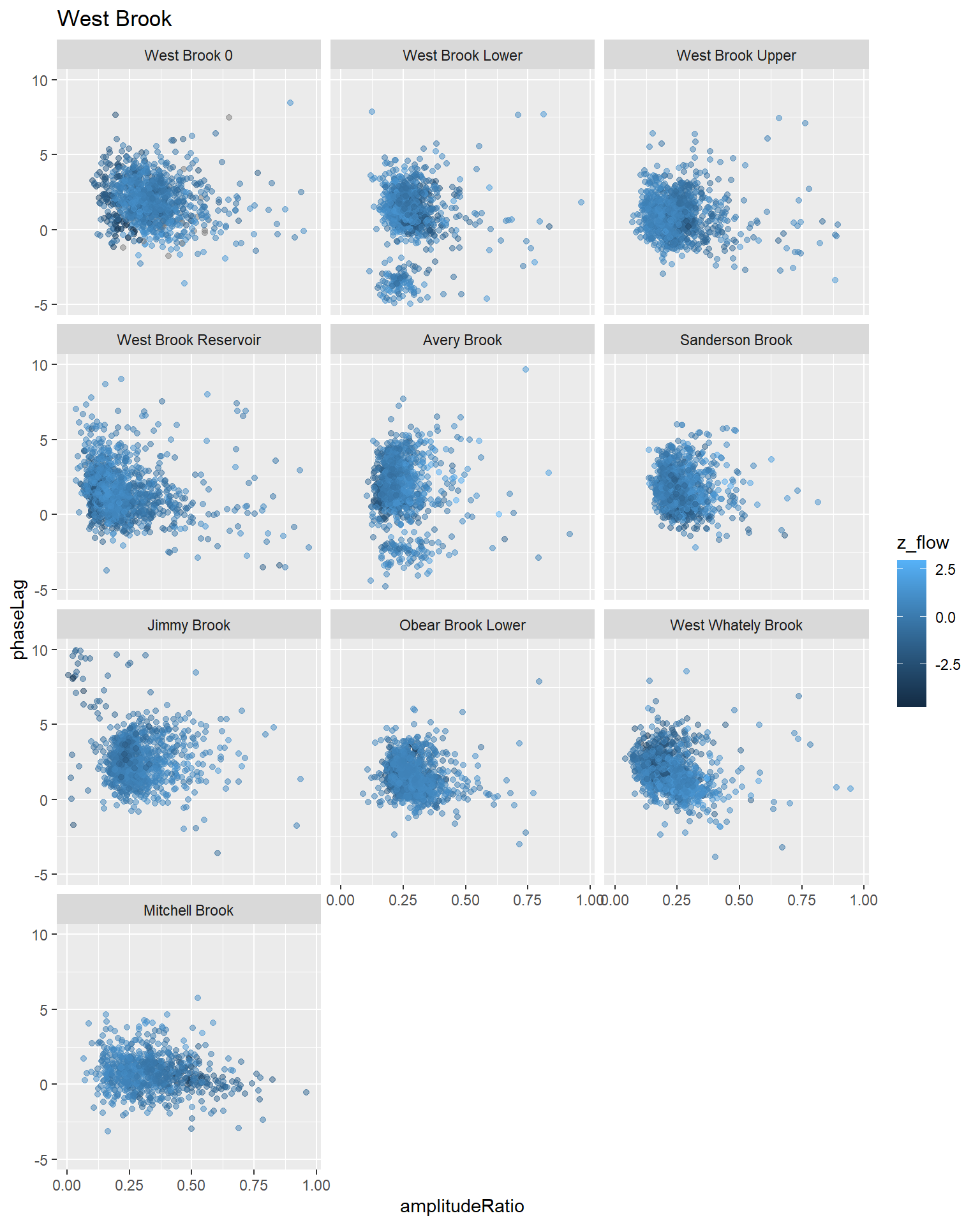
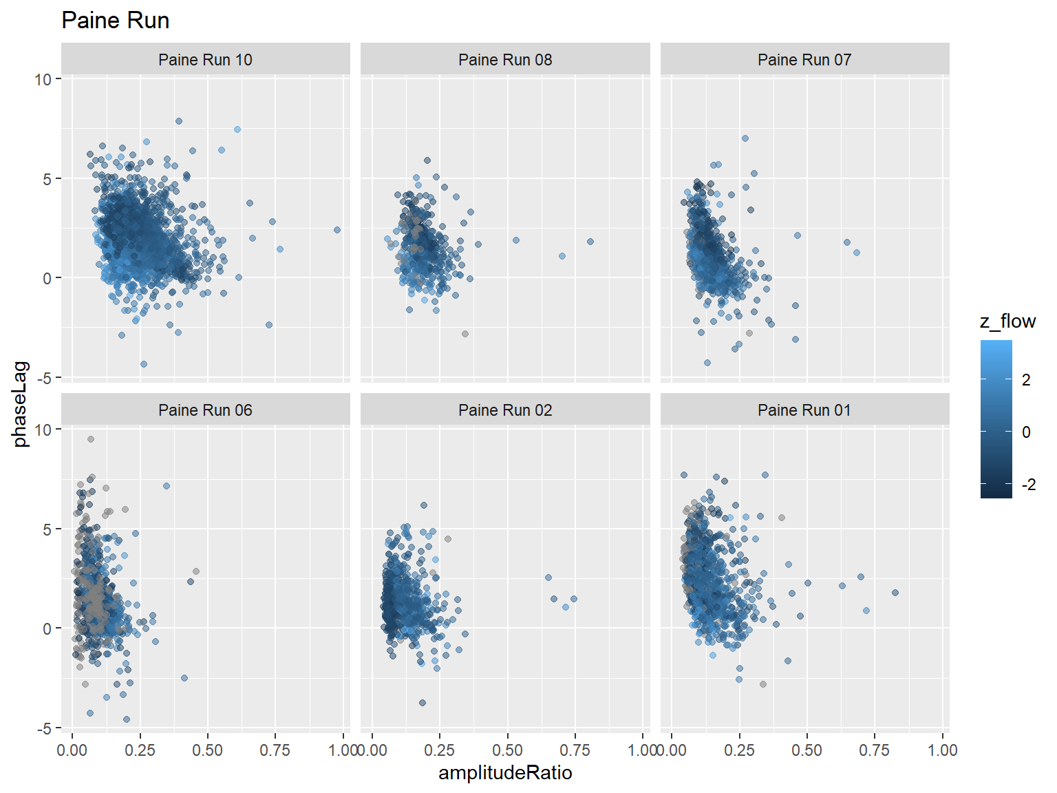
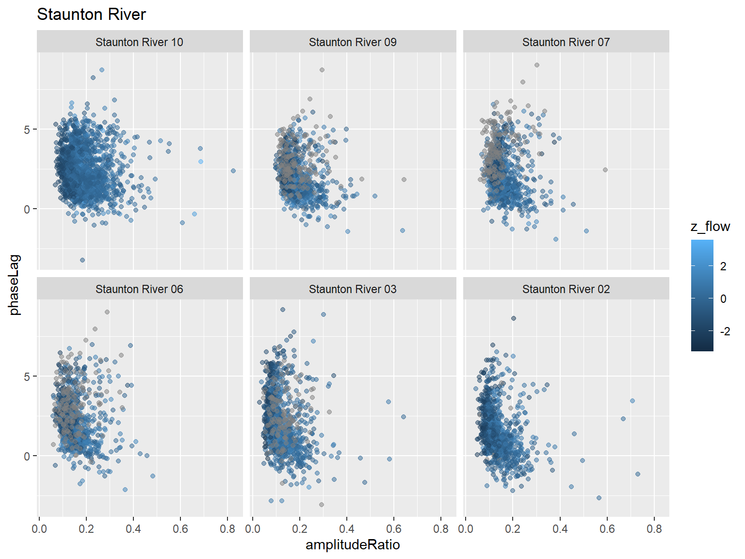
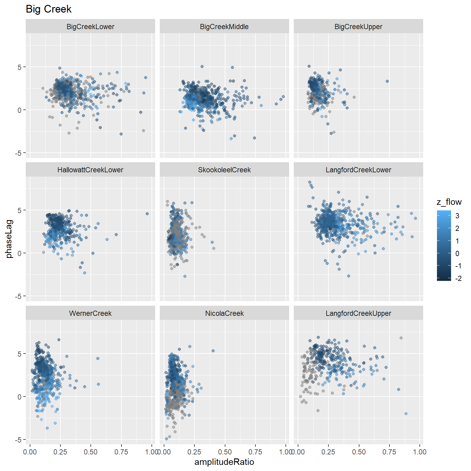
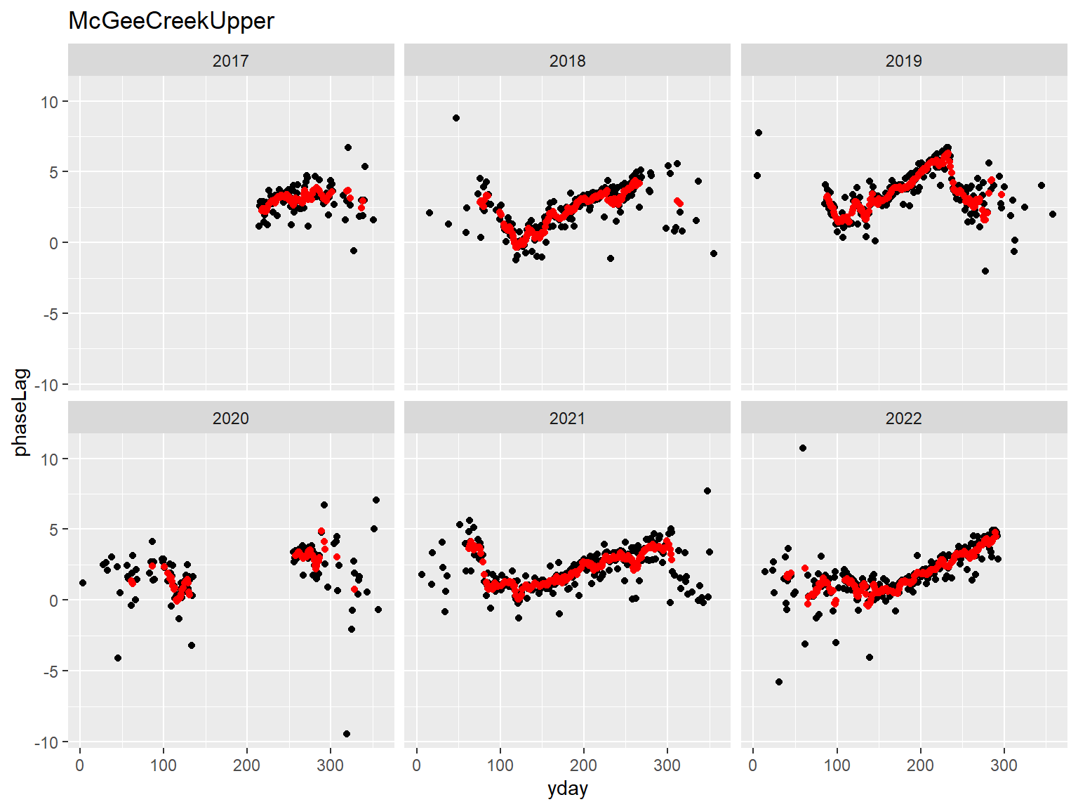
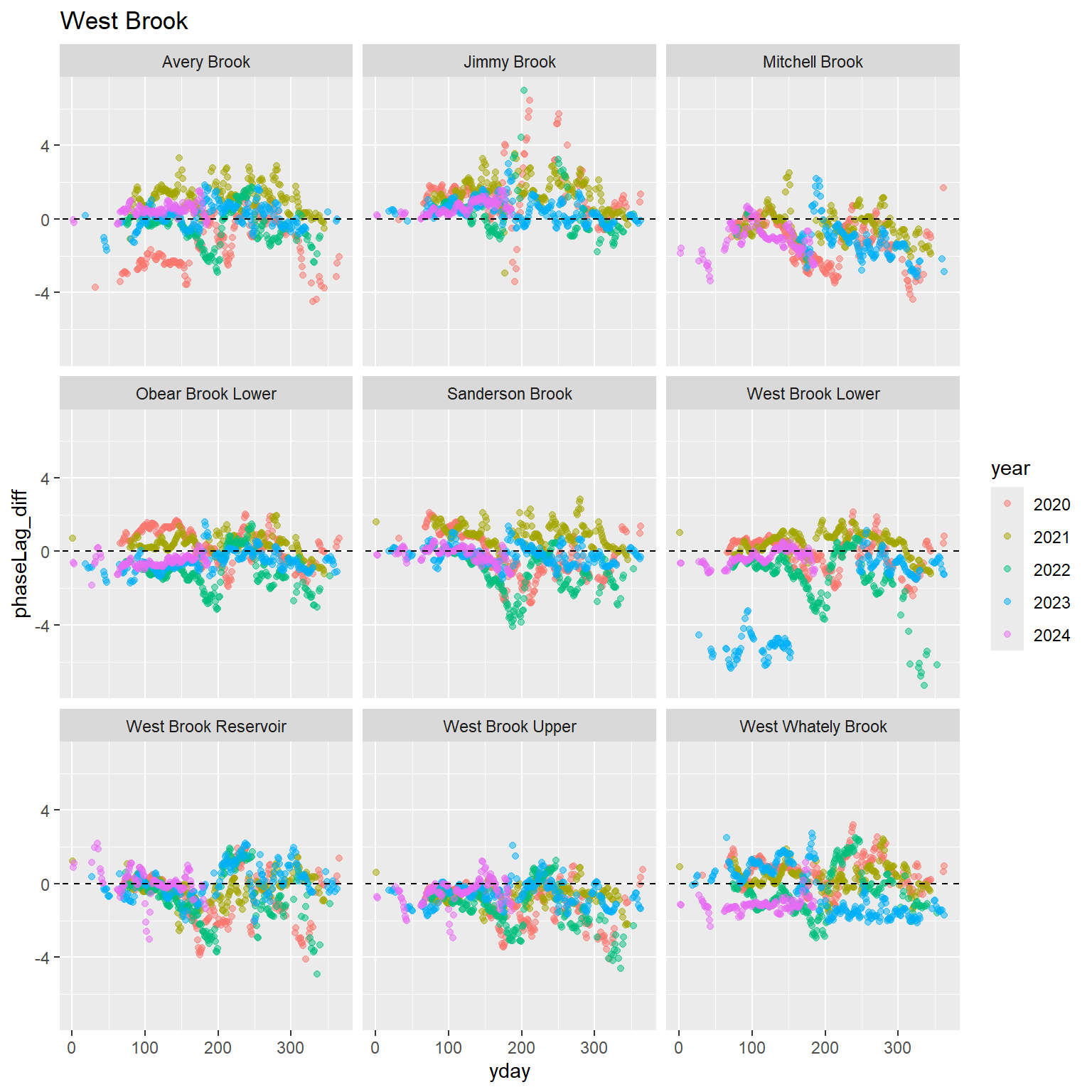
Phase lag: phase_water - phase_air. Phase lags are likely a result of diel groundwater temperature variations that are subsequently transferred to water temperatures signals. Generally, phase lag tends to be inversely related to amplitude ratio and may provide a secondary metric of fractional groundwater contributions.

pasta_derived %>% filter(site_name == focal_site, rSquared_air >= 0.7 & rSquared_water >= 0.7) %>% select(date, phaseLag) %>% dygraph(main = focal_site) %>% dyRangeSelector() %>% dyAxis("y", label = "Phase lag (hrs)") %>% dyOptions(drawPoints = T, strokeWidth = 0, pointSize = 3) %>% dyLimit(0, color = "red") %>% dyHighlight(highlightCircleSize = 5)

pasta_derived %>% filter(site_name == focal_site, rSquared_air >= 0.7 & rSquared_water >= 0.7) %>% ggplot(aes(x = yday, y = phaseLag, color = z_flow)) + geom_point() + ggtitle(focal_site) + geom_smooth() + facet_wrap(~year)

pasta_derived %>% filter(site_name == focal_site, rSquared_air >= 0.7 & rSquared_water >= 0.7) %>% ggplot(aes(x = z_flow, y = phaseLag, color = as.factor(year))) + geom_point(alpha= 0.3) + ggtitle(focal_site) + geom_smooth(se = FALSE)

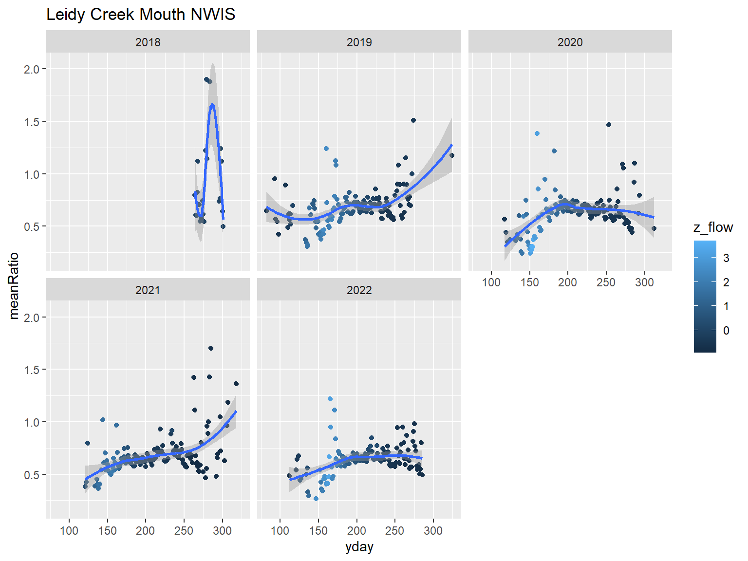
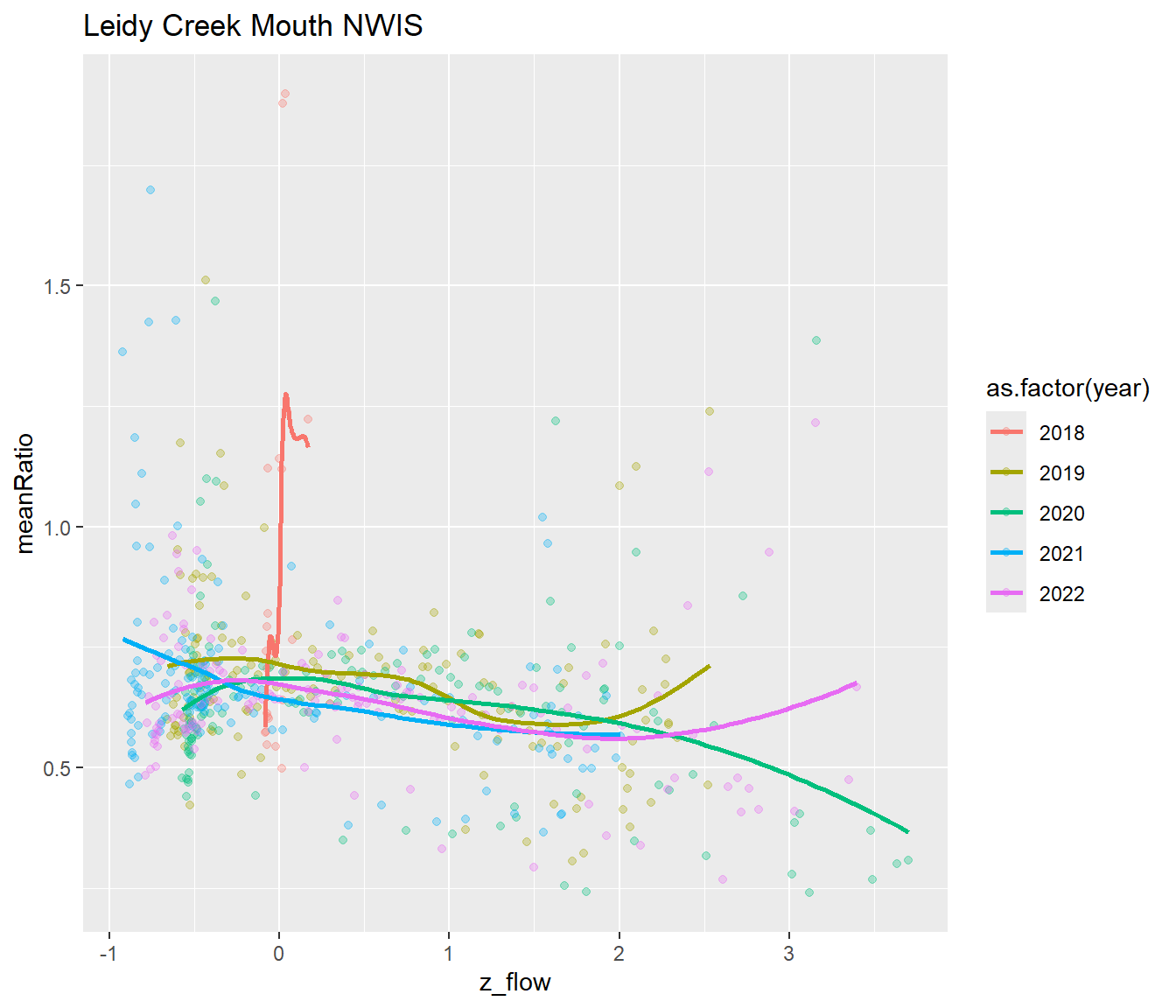
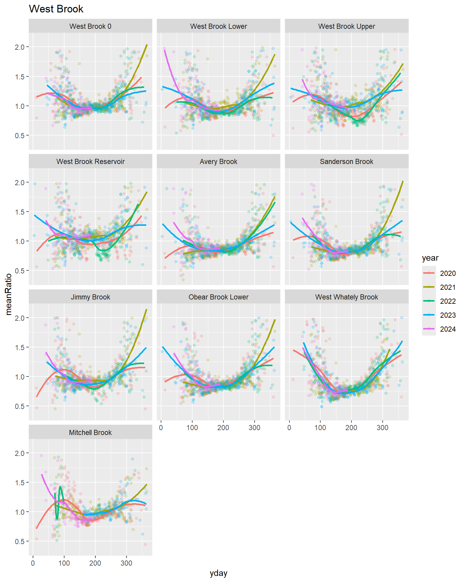
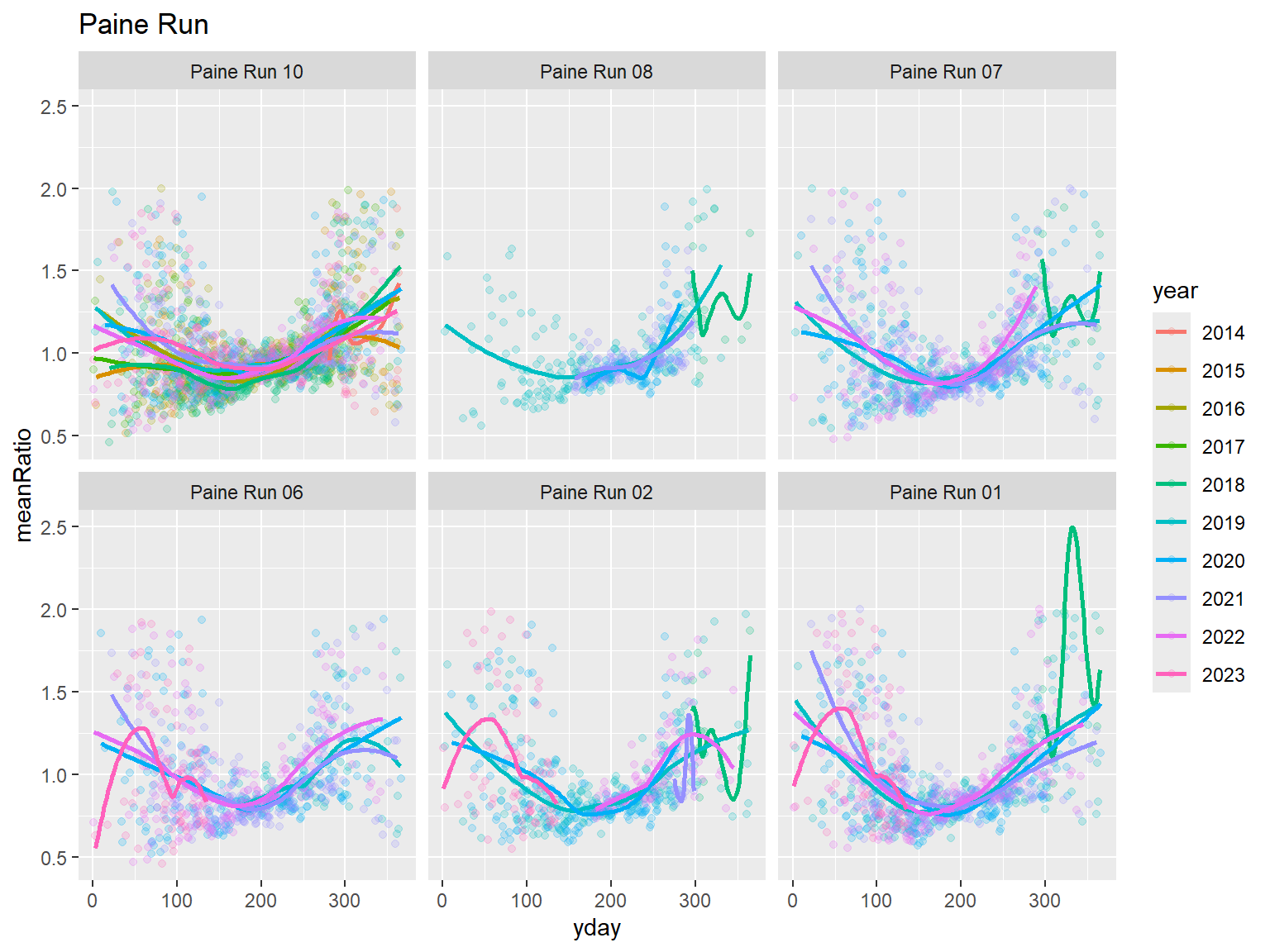
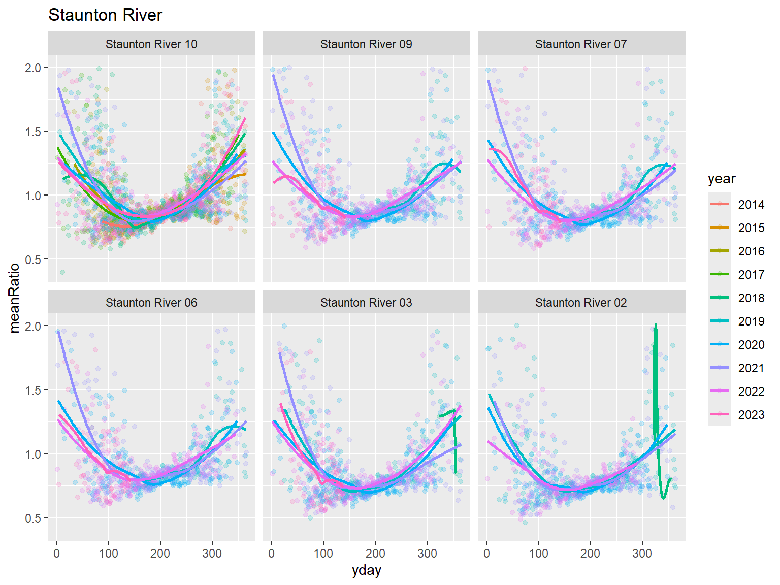
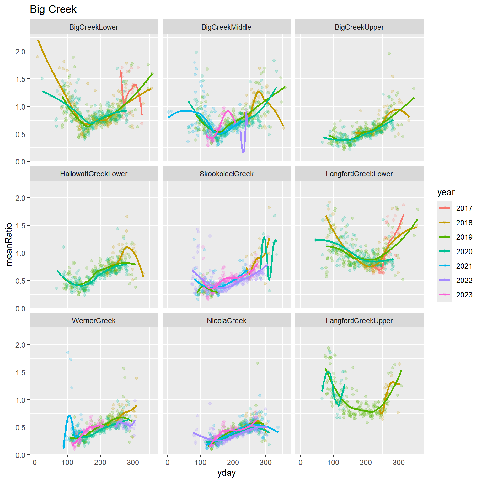
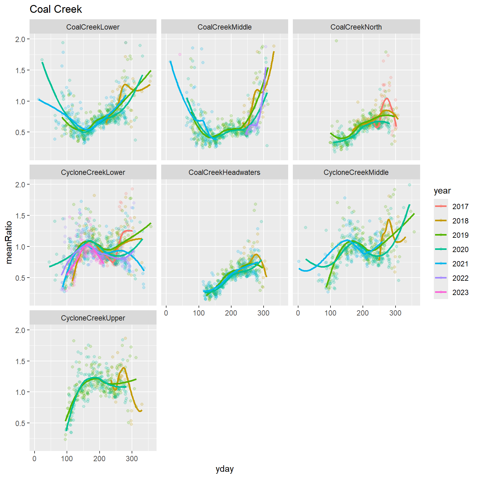
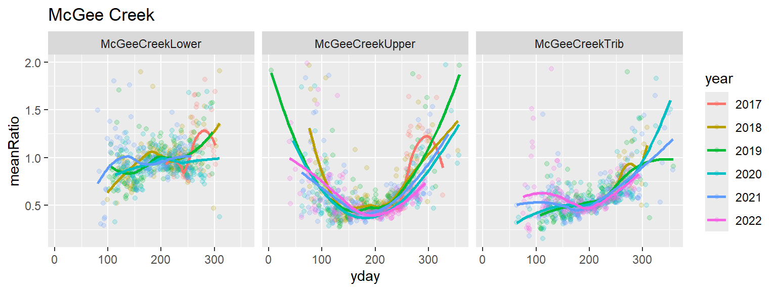
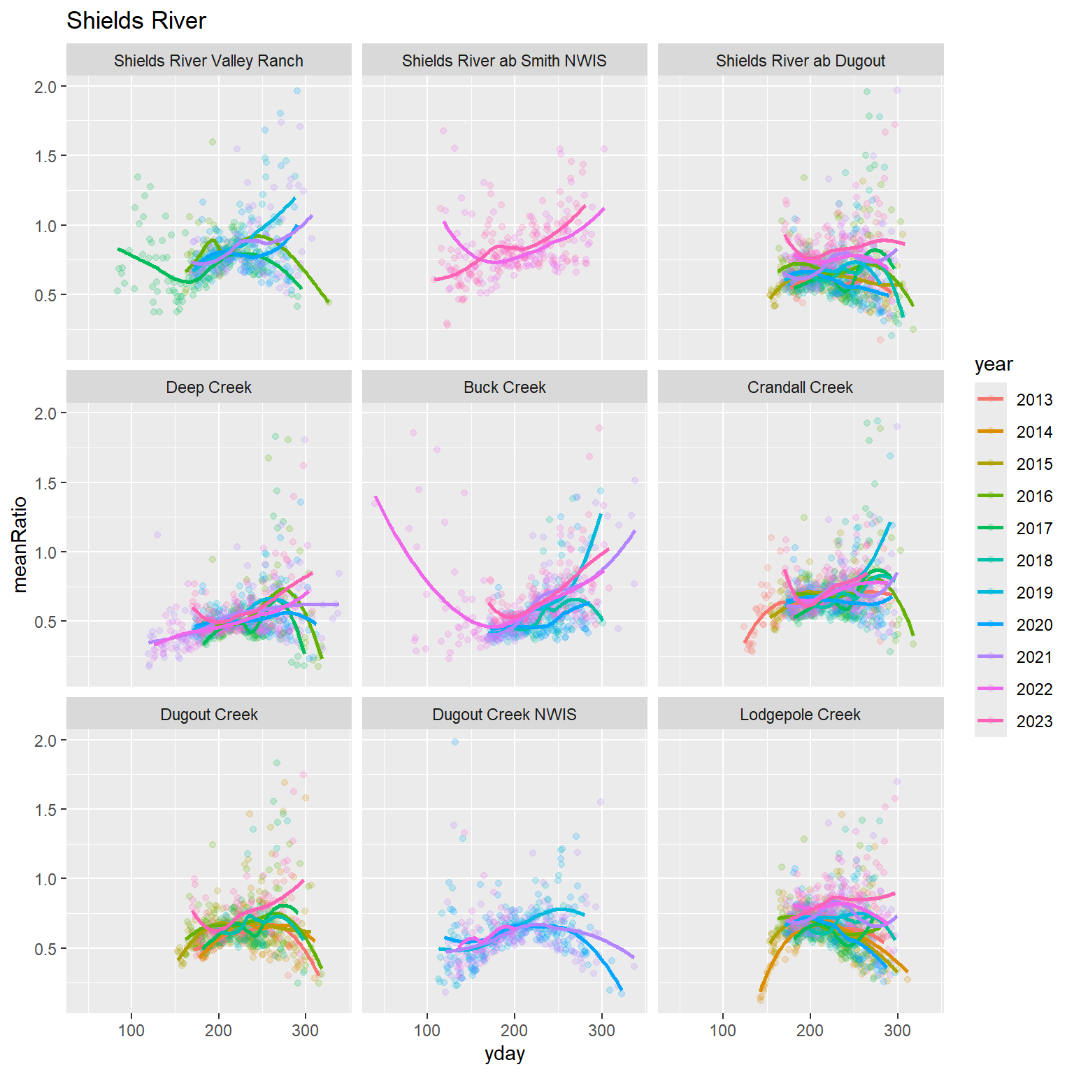
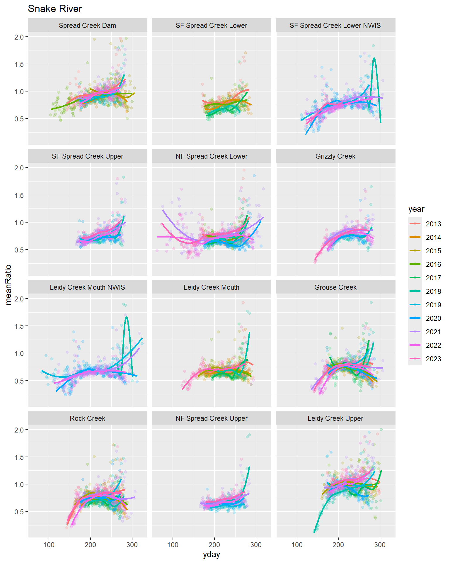
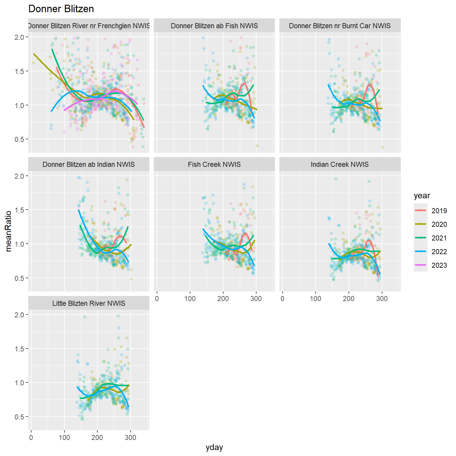
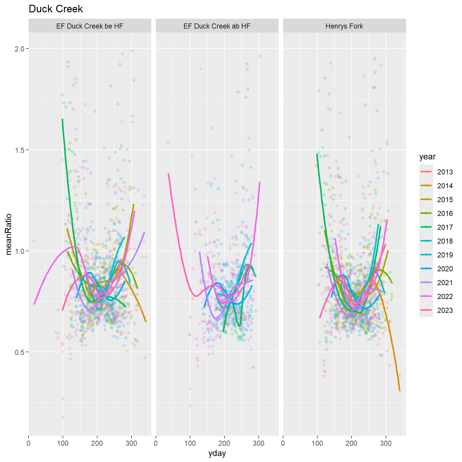
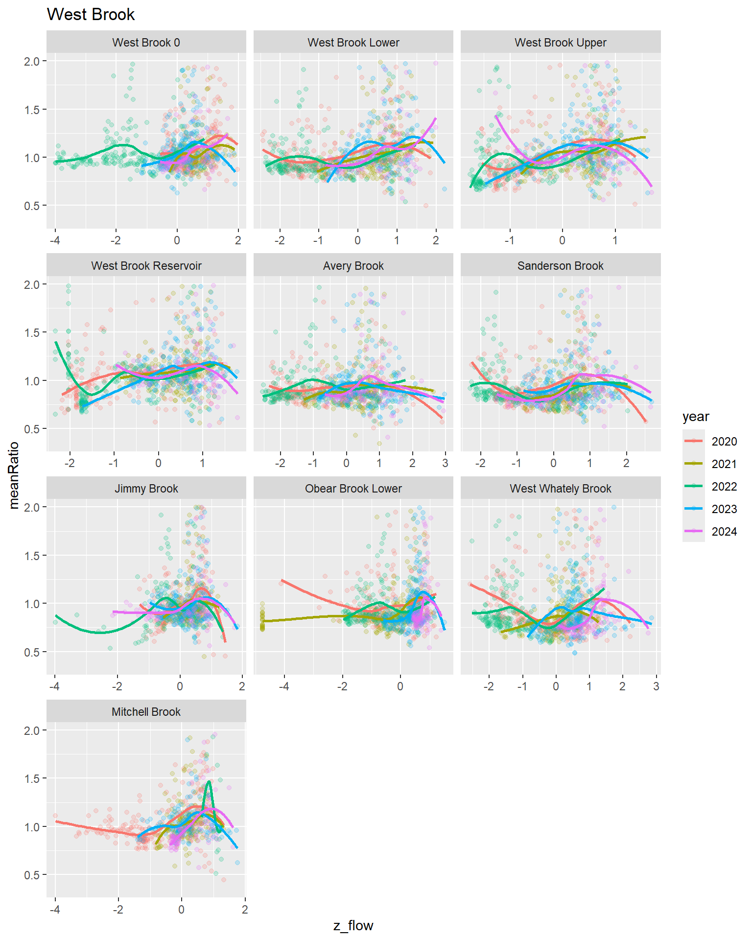
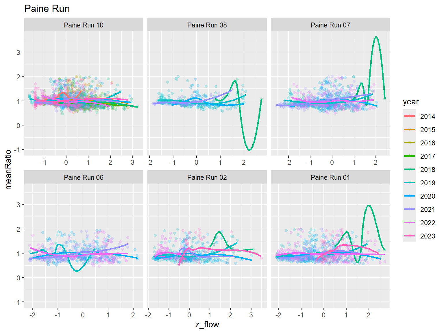
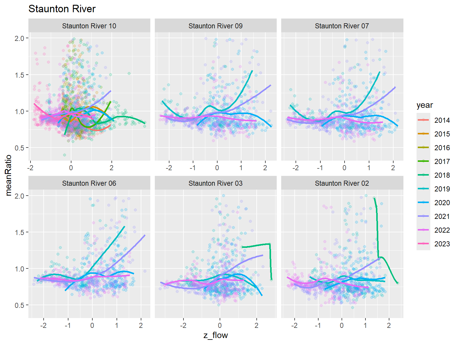
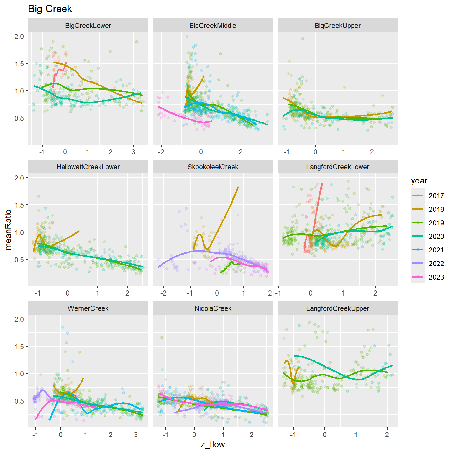
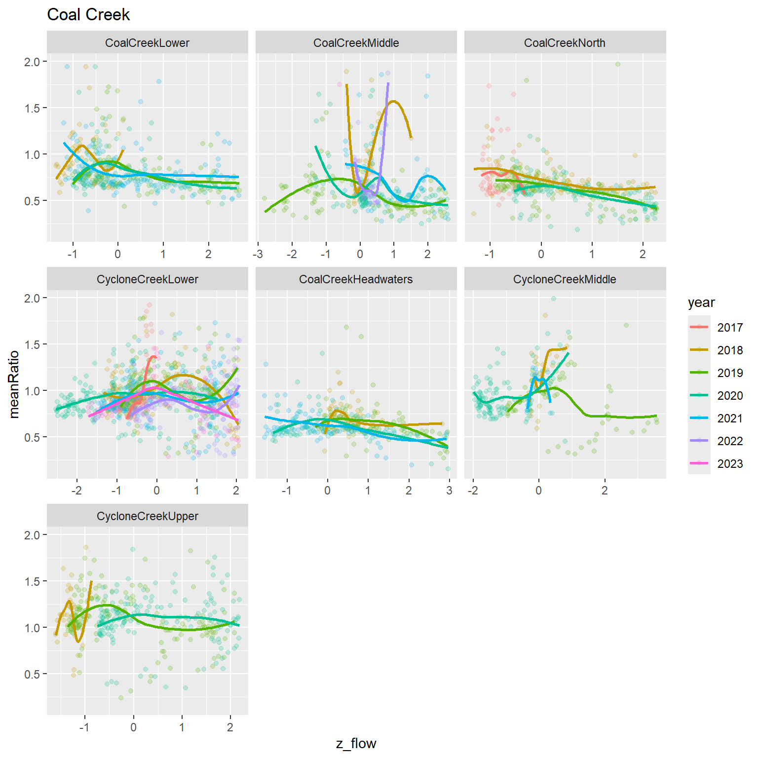
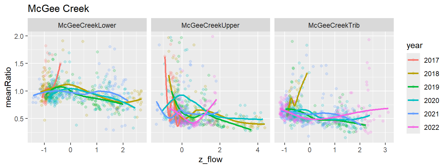
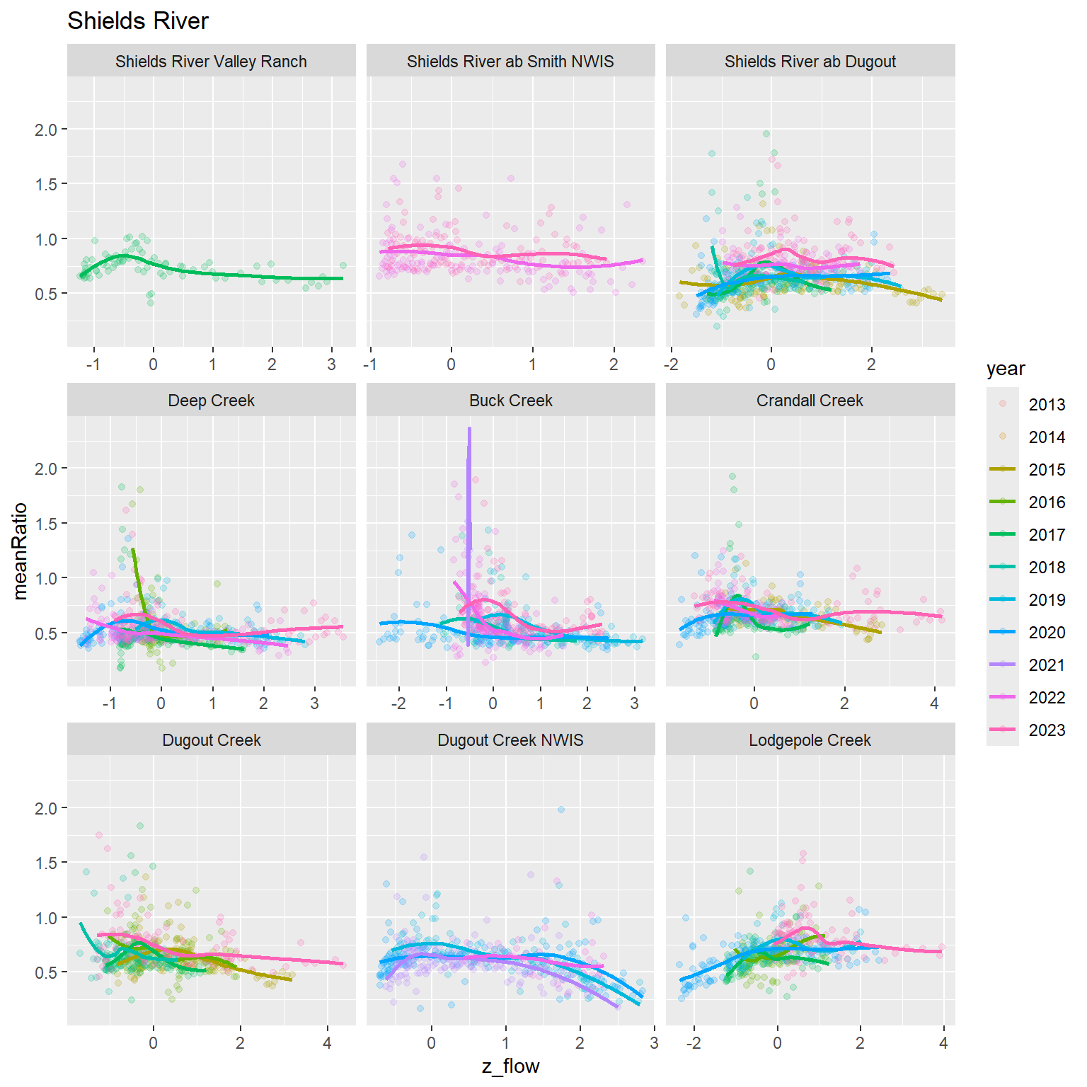
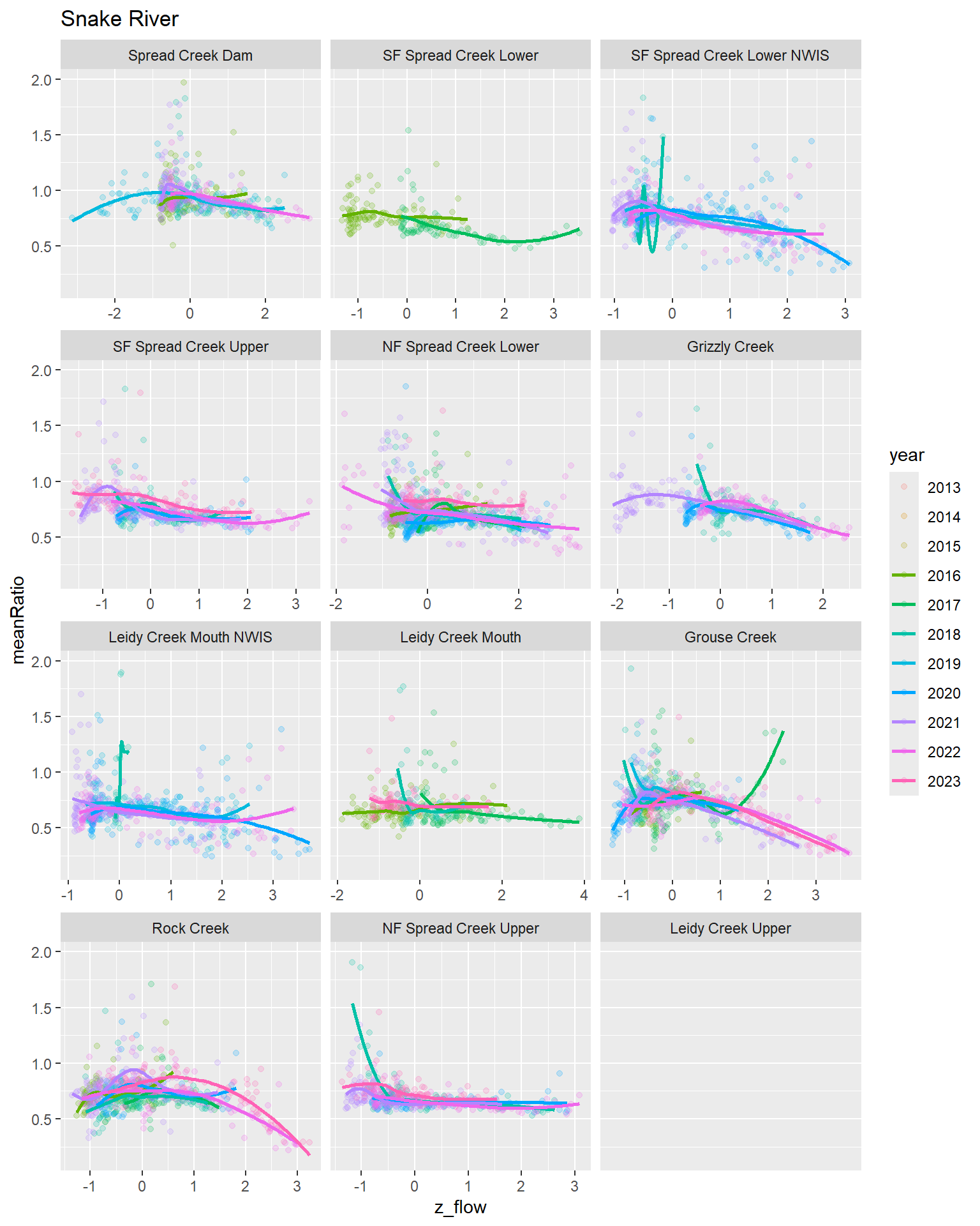
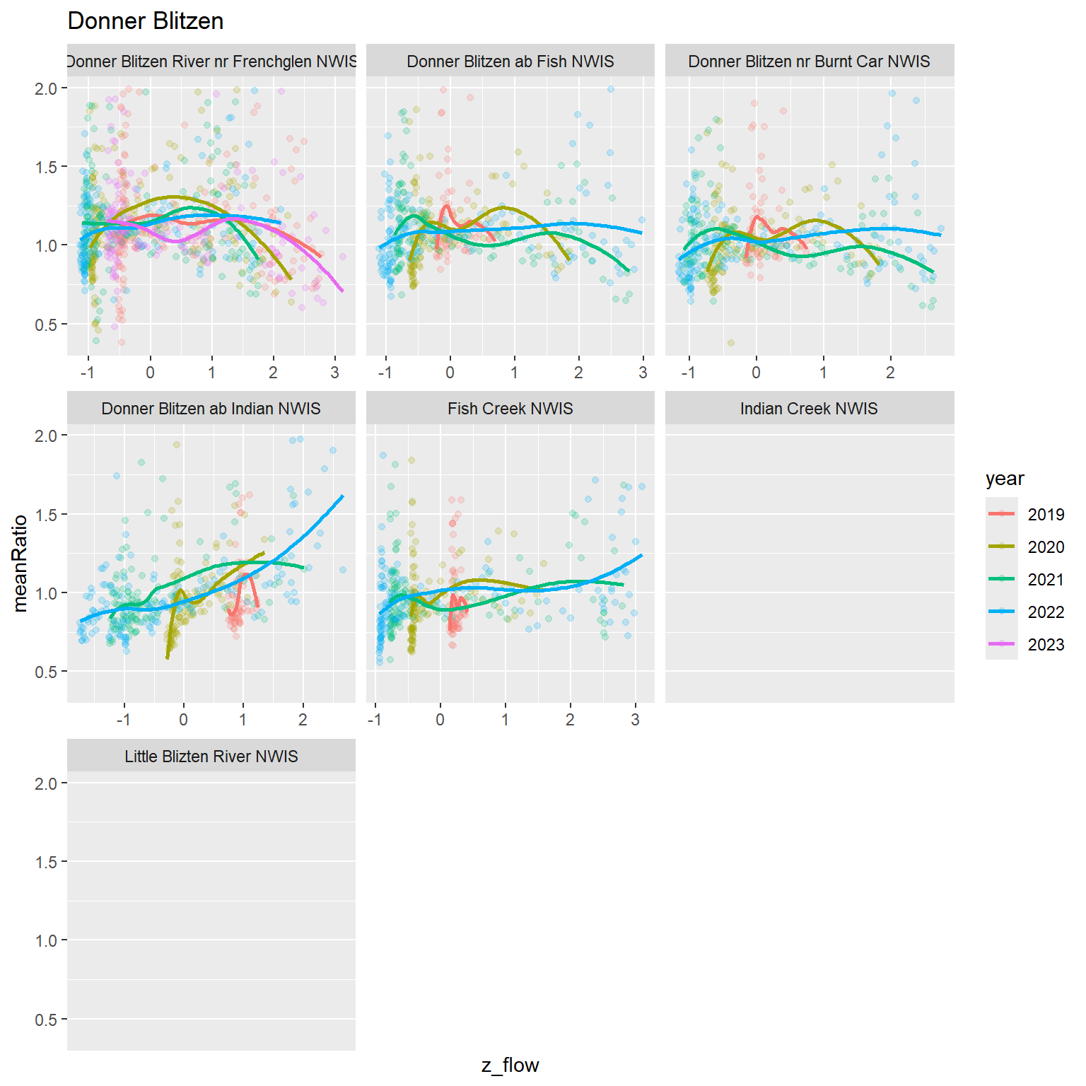
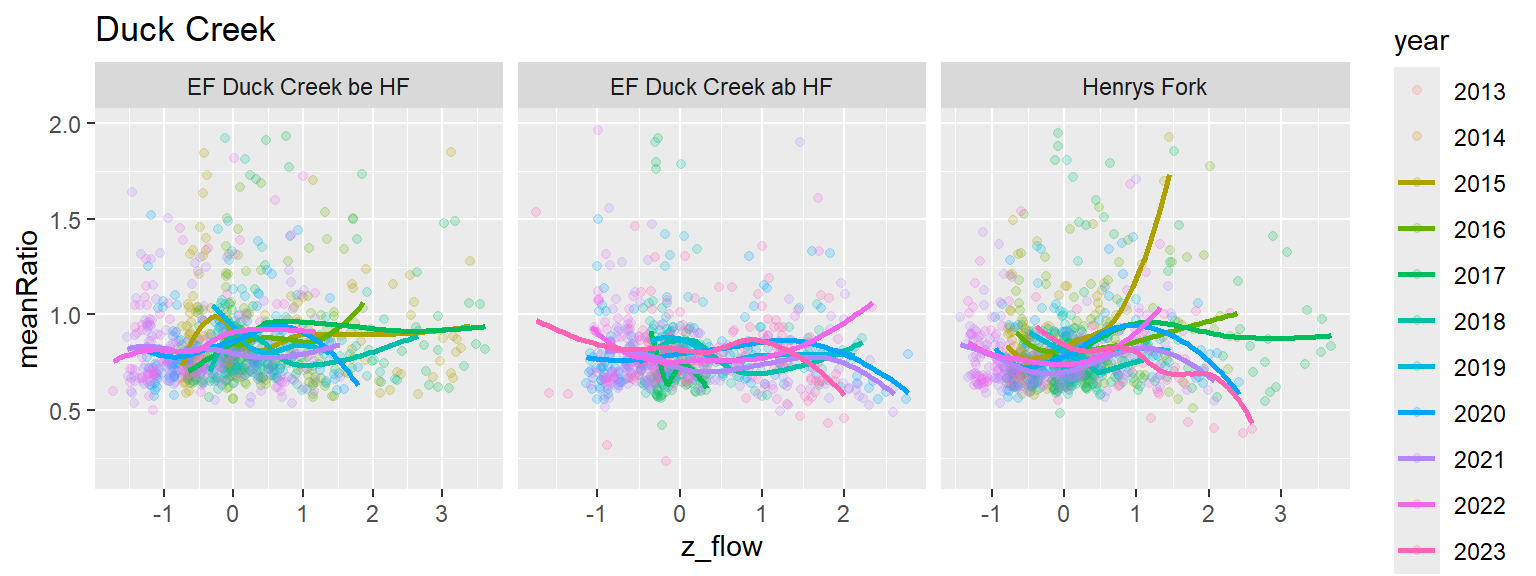
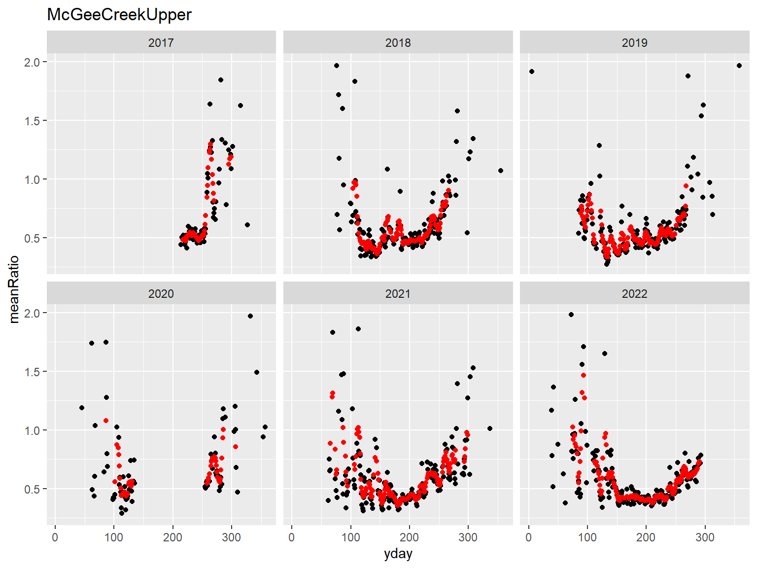
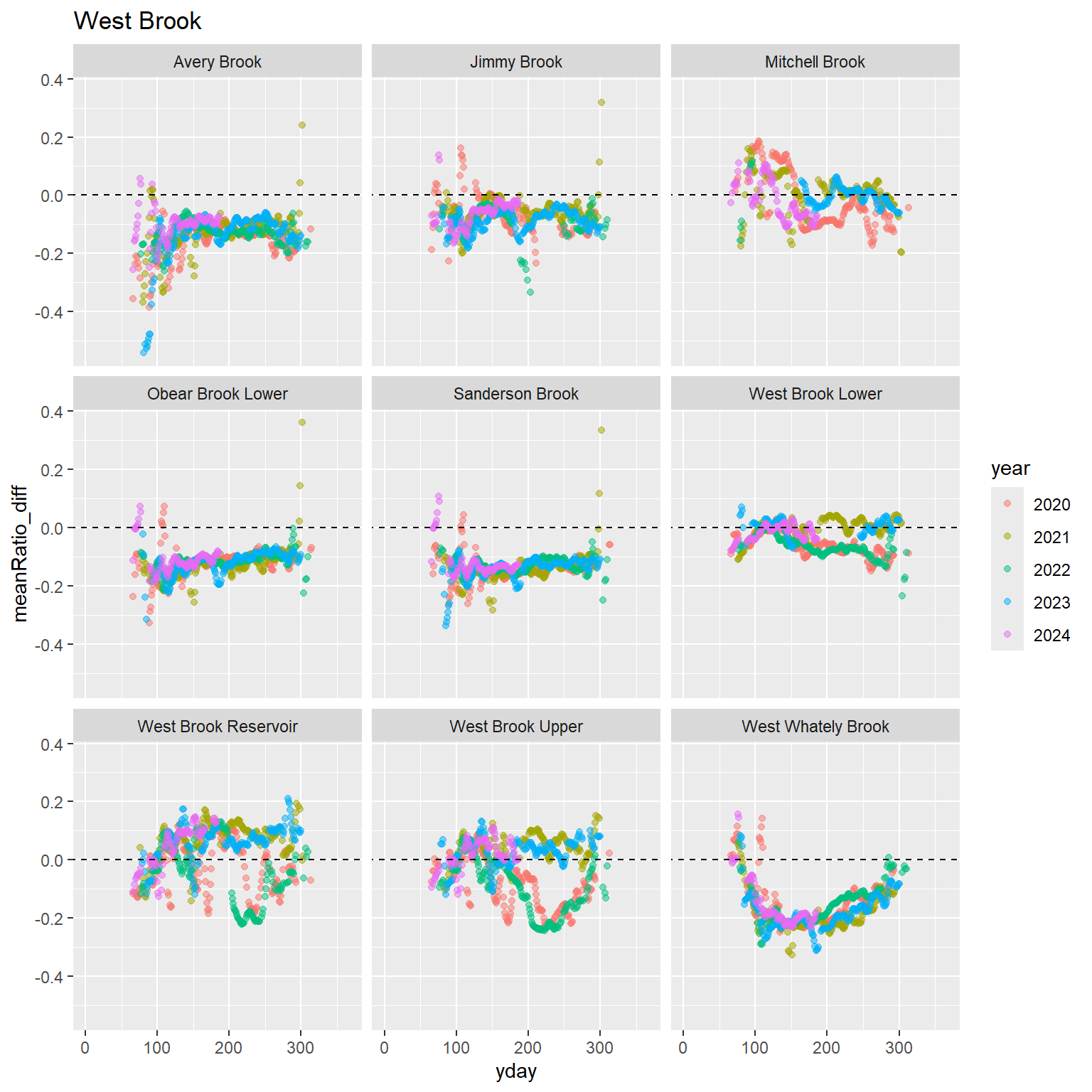
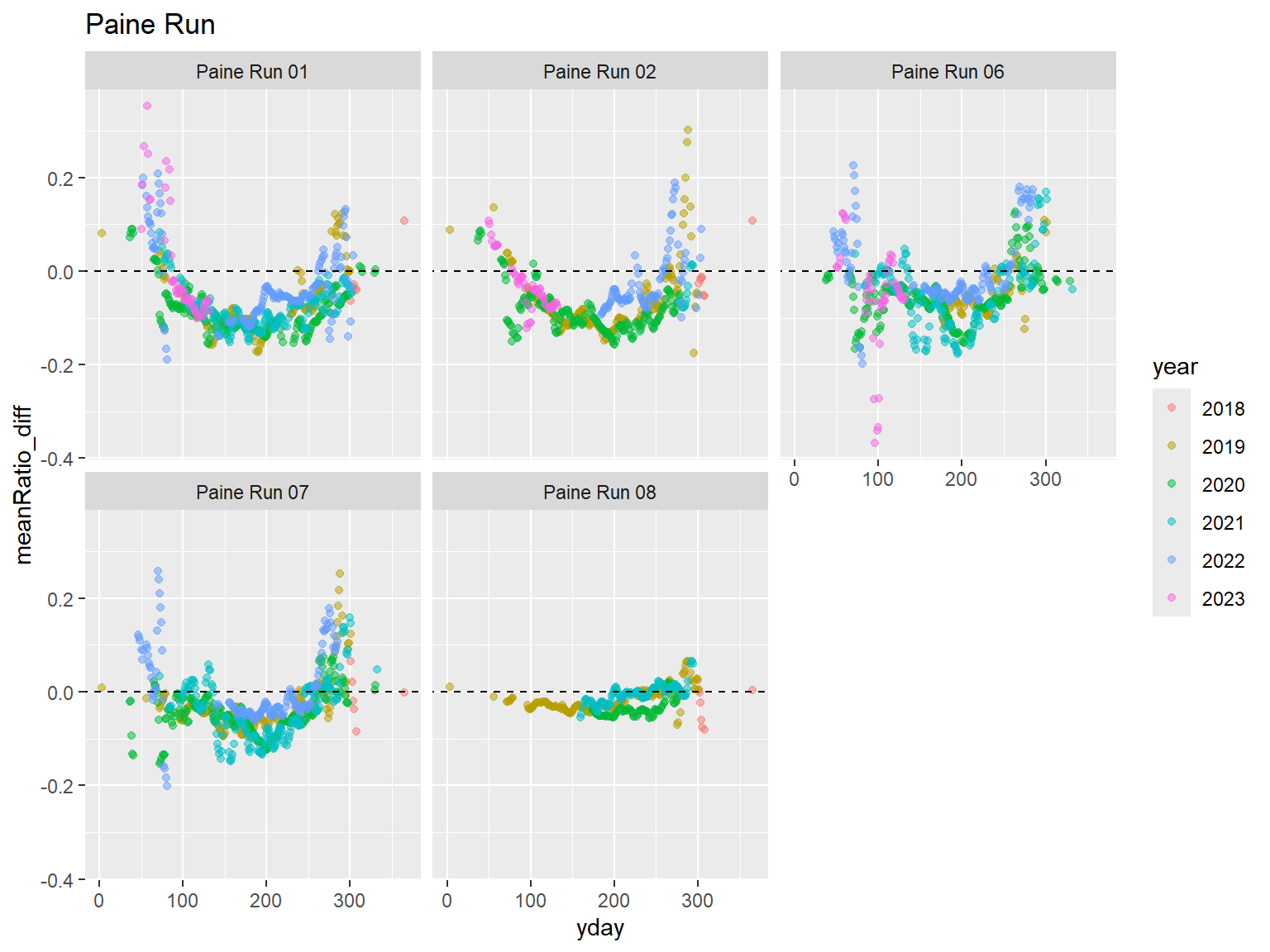
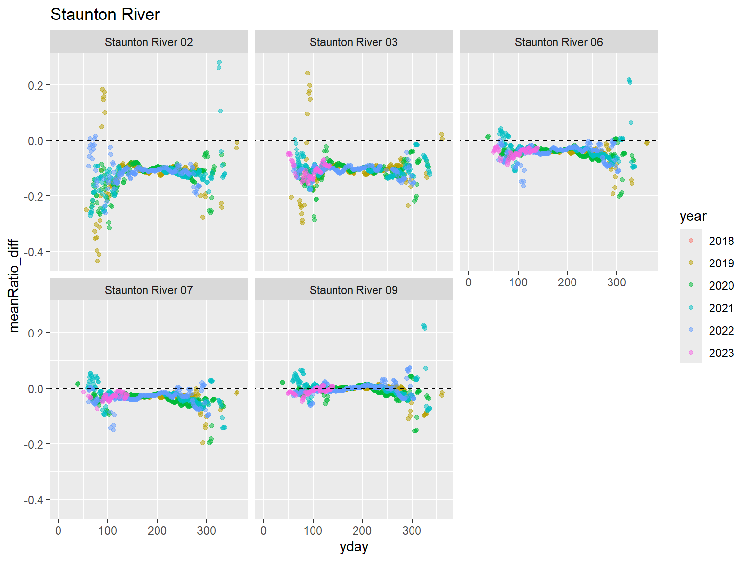
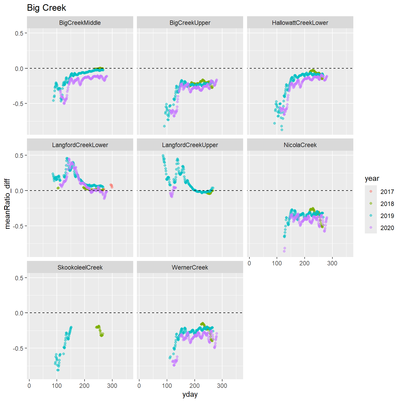
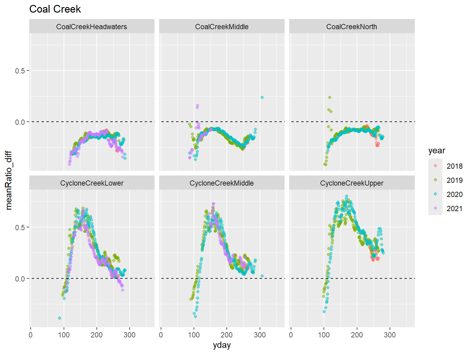
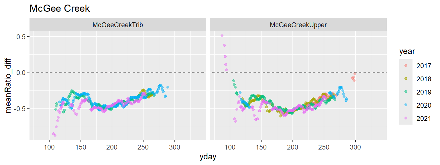
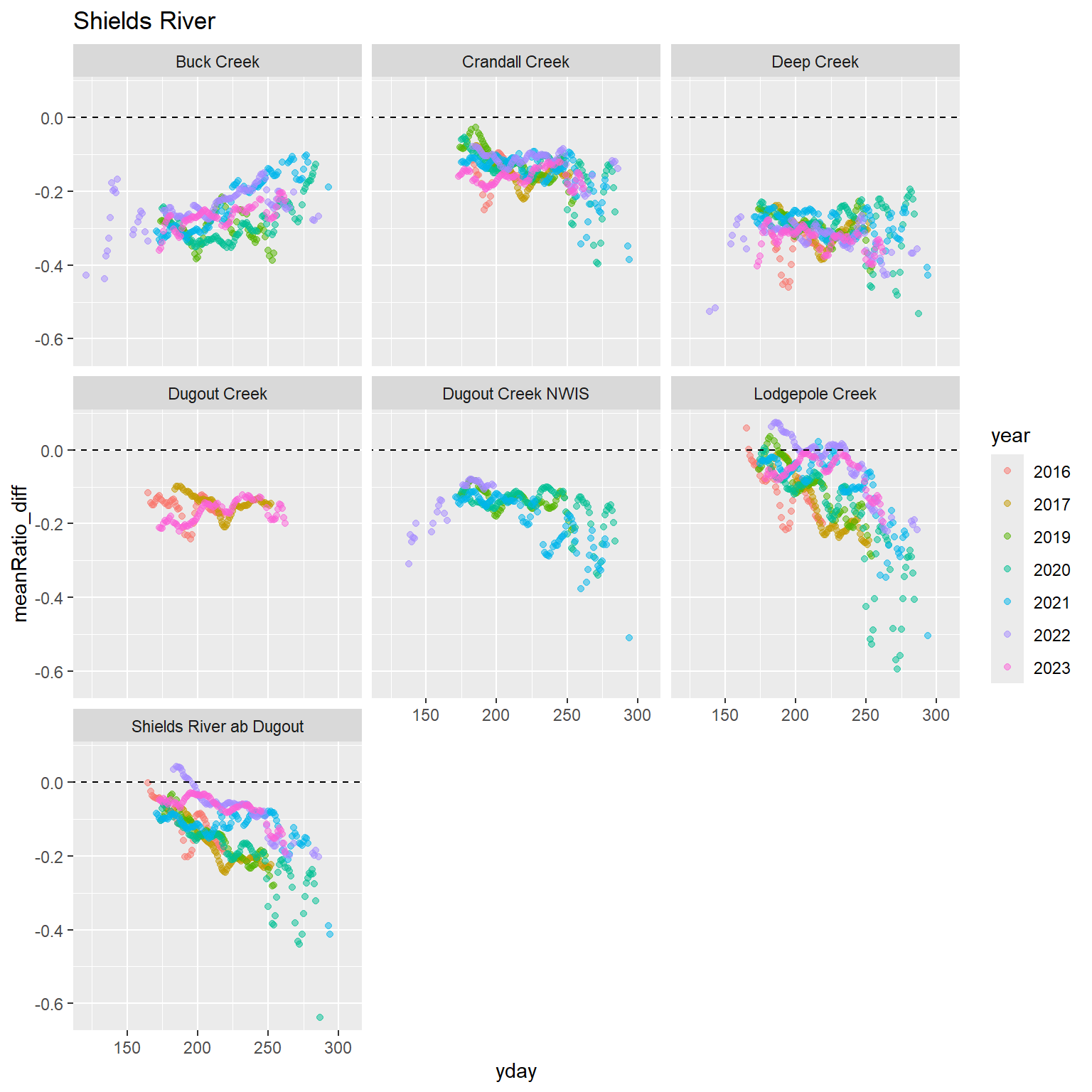
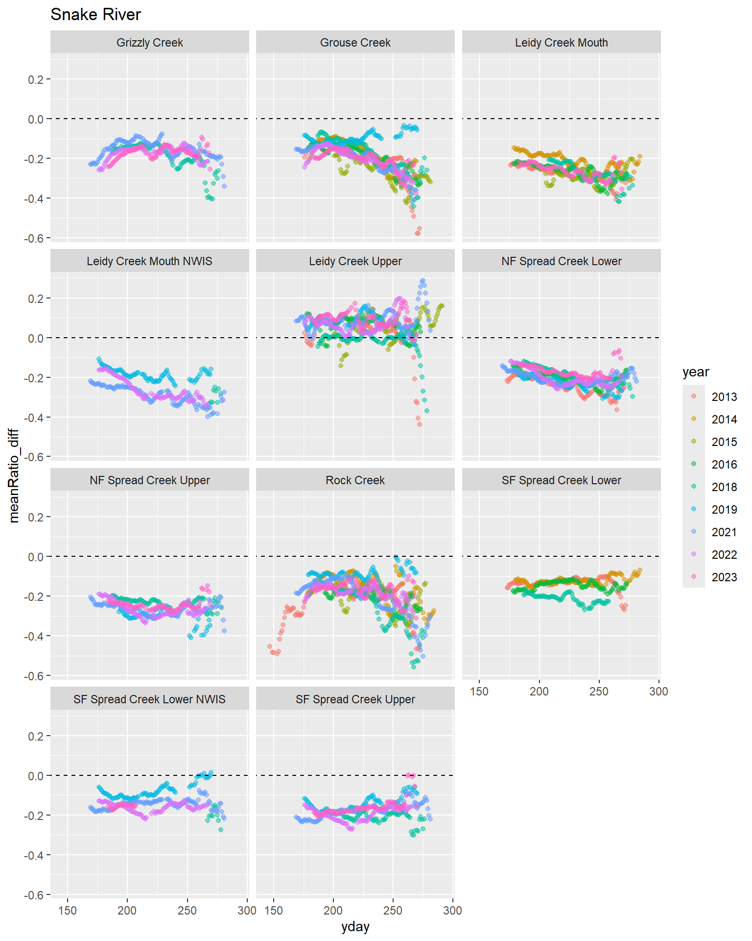
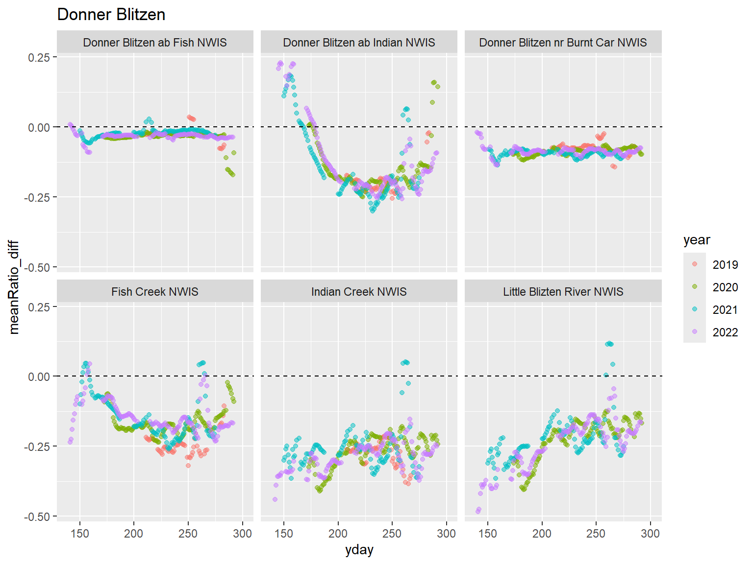
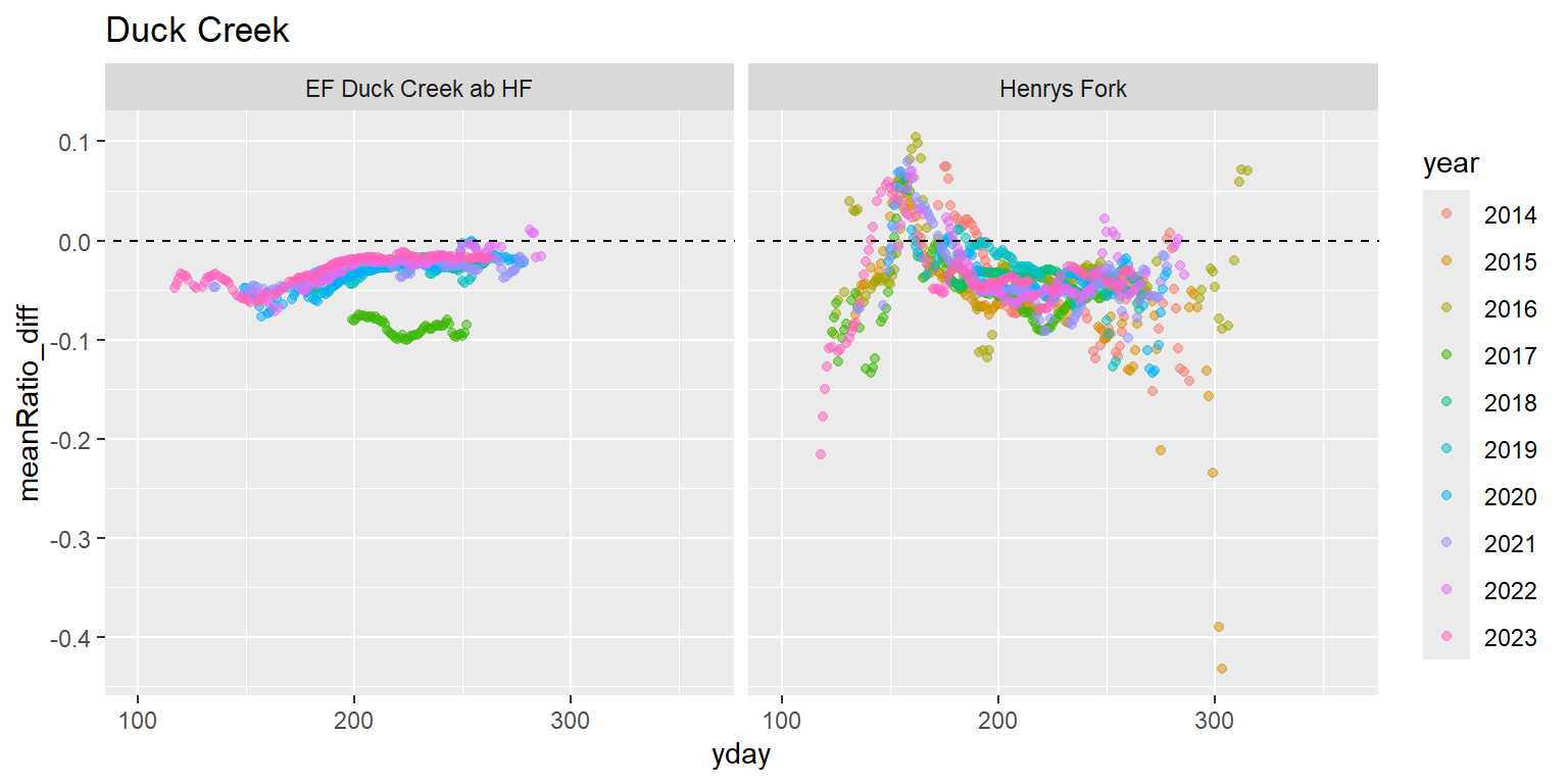
7.4.1.3 Mean ratio

Mean ratio: mean_water / mean_air. On daily timescales, mean ratio values indicate runoff/quickflow vs. local groundwater influence, with higher, more stable values at sites where hillslope drainage is reduced compared to total channel water volume (e.g., lower in network). I.e., across sites at any given time, low values indicate high fractional groundwater input and high values indicate low groundwater input. Within a site across time, gradual rise/change in Mr may be driven by changes in groundwater temperature over time as terrestrial hillslopes accumulate (spring and early summer) and/or lose (late summer and autumn) heat. Thereby indicating that groundwater flowpaths are shallow enough to be sensitive to seasonal warming/cooling.

(In Rey et al. 2024, Mr values tend to be most similar among tributary/mainstem sites during periods of high surface water input. I.e., high flows homogenize spatial variation in groundwater-surface water dynamics).

Note this plot is trimmed to values [0,2] as very unreasonable values can result when daily mean air temperature is < 1.

pasta_derived %>% filter(site_name == focal_site, rSquared_air >= 0.7, rSquared_water >= 0.7, meanRatio >=0, meanRatio <= 2) %>% select(date, meanRatio) %>% dygraph(main = focal_site) %>% dyRangeSelector() %>% dyAxis("y", label = "Mean ratio") %>% dyOptions(drawPoints = T, strokeWidth = 0, pointSize = 3) %>% dyHighlight(highlightCircleSize = 5)

pasta_derived %>% filter(site_name == focal_site, rSquared_air >= 0.7 & rSquared_water >= 0.7, meanRatio >=0, meanRatio <= 2) %>% ggplot(aes(x = yday, y = meanRatio, color = z_flow)) + geom_point() + ggtitle(focal_site) + geom_smooth() + facet_wrap(~year)

pasta_derived %>% filter(site_name == focal_site, rSquared_air >= 0.7 & rSquared_water >= 0.7, meanRatio >=0, meanRatio <= 2) %>% ggplot(aes(x = z_flow, y = meanRatio, color = as.factor(year))) + geom_point(alpha= 0.3) + ggtitle(focal_site) + geom_smooth(se = FALSE)

7.4.1.4 Pl-Ar correlation

In Rey et al. 2024, phase lag and amplitude ratio are often correlated.

pasta_derived %>% filter(site_name == focal_site, rSquared_air >= 0.7 & rSquared_water >= 0.7) %>% ggplot(aes(x = amplitudeRatio, y = phaseLag, color = z_flow)) + geom_point() + ggtitle(focal_site) + geom_smooth(method = "lm") + facet_wrap(~year)

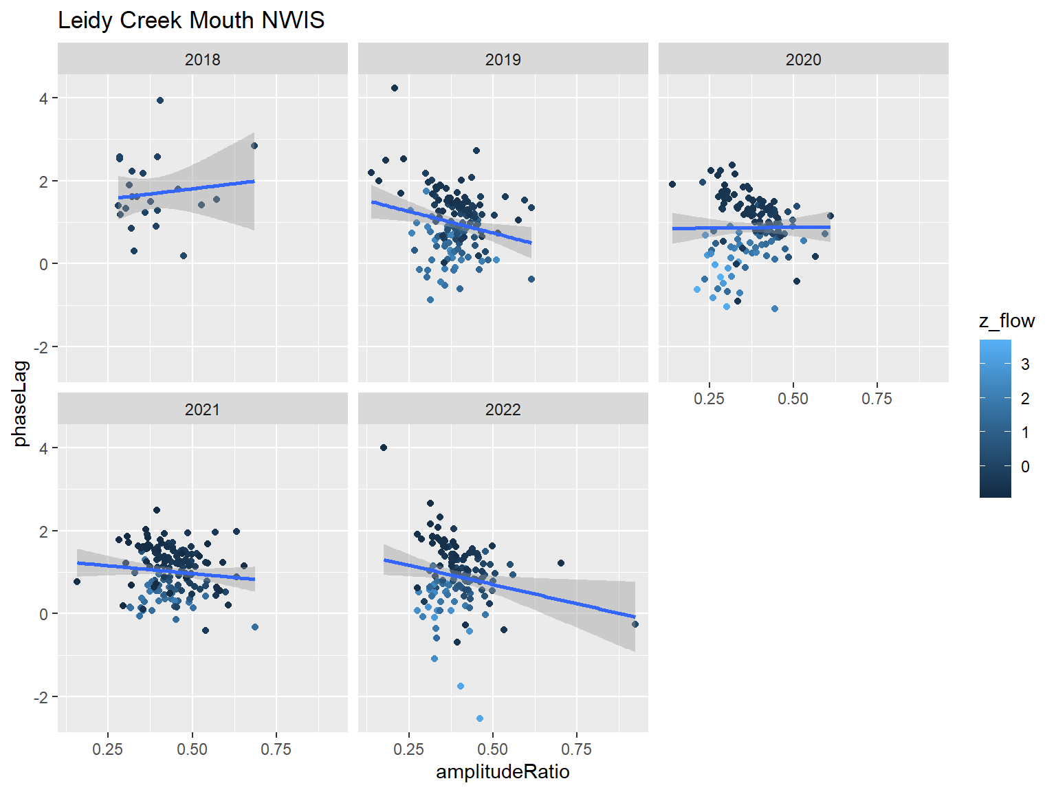
This simple OLS model shows that phase lag is negatively related to both amplitude ratio and flow. I.e., the intercept of the Pl ~ Ar relationship declines with increasing streamflow.

summary(lm(phaseLag ~ amplitudeRatio*z_flow, pasta_derived %>% filter(site_name == focal_site, rSquared_air >= 0.7 & rSquared_water >= 0.7)))

Call:
lm(formula = phaseLag ~ amplitudeRatio * z_flow, data = pasta_derived %>% 
    filter(site_name == focal_site, rSquared_air >= 0.7 & rSquared_water >= 
        0.7))

Residuals:
     Min       1Q   Median       3Q      Max 
-2.39573 -0.21486  0.02893  0.24727  2.79277 

Coefficients:
                      Estimate Std. Error t value Pr(>|t|)    
(Intercept)            1.91249    0.10844  17.636  < 2e-16 ***
amplitudeRatio        -1.92841    0.26245  -7.348 6.72e-13 ***
z_flow                -0.60032    0.09622  -6.239 8.39e-10 ***
amplitudeRatio:z_flow  0.34113    0.25958   1.314    0.189    
---
Signif. codes:  0 '***' 0.001 '**' 0.01 '*' 0.05 '.' 0.1 ' ' 1

Residual standard error: 0.5195 on 592 degrees of freedom
Multiple R-squared:  0.4858,    Adjusted R-squared:  0.4832 
F-statistic: 186.4 on 3 and 592 DF,  p-value: < 2.2e-16

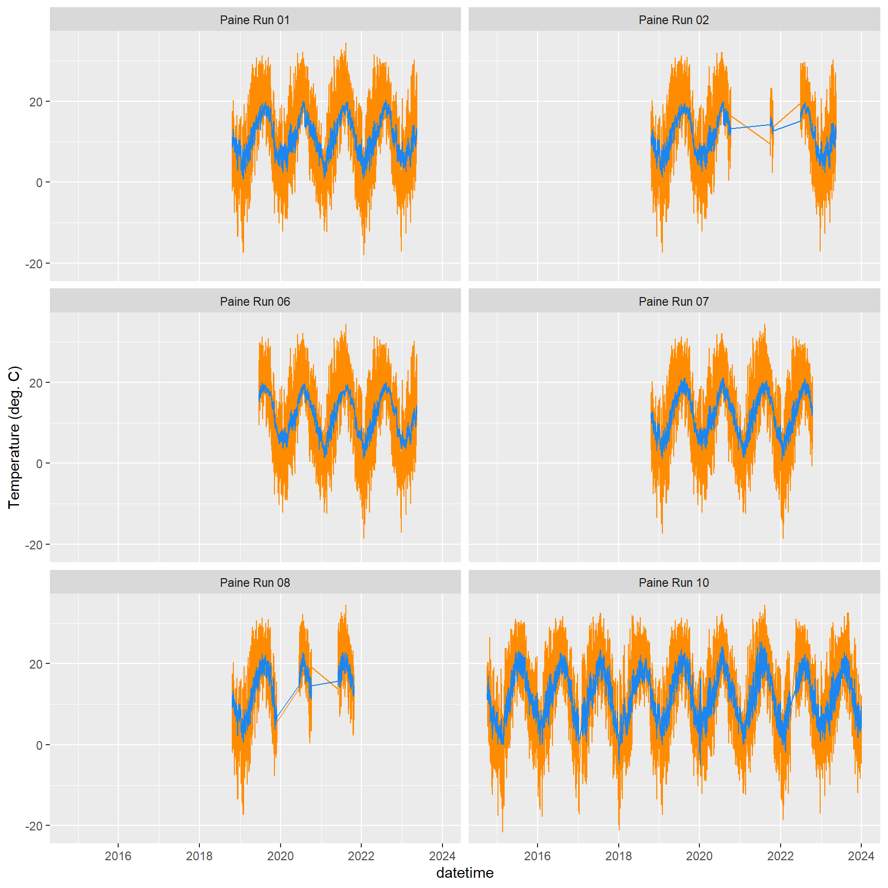
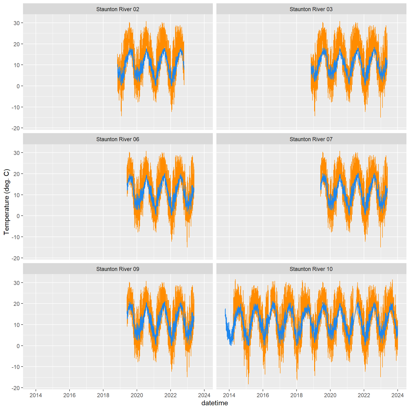
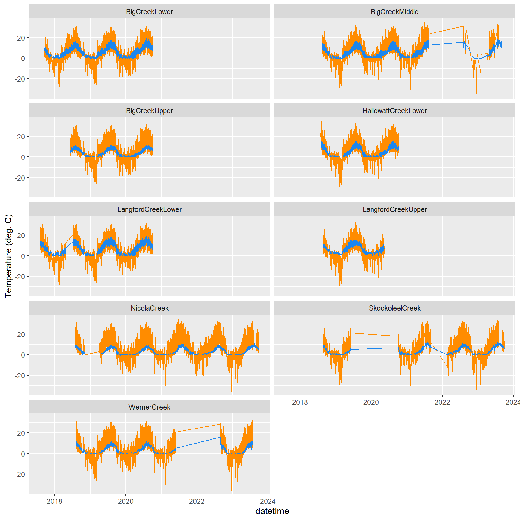
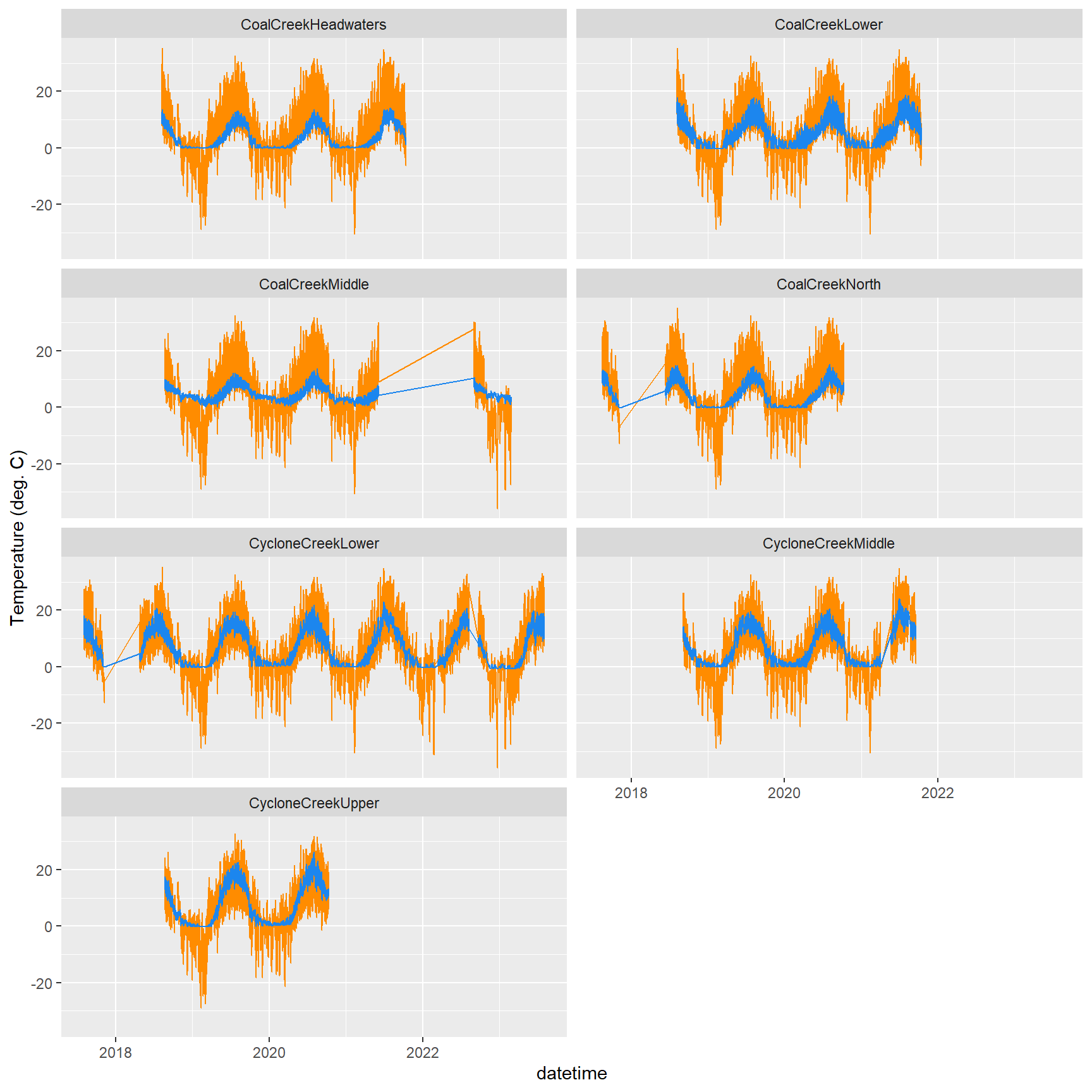
7.4.1.5 Model predictions

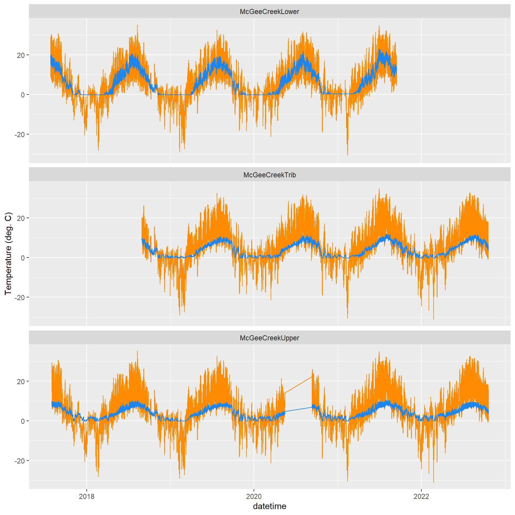
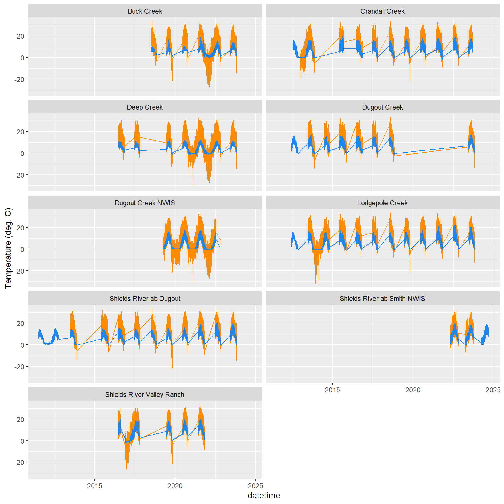
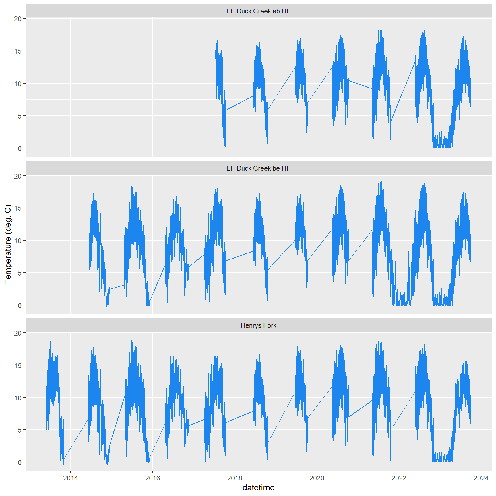
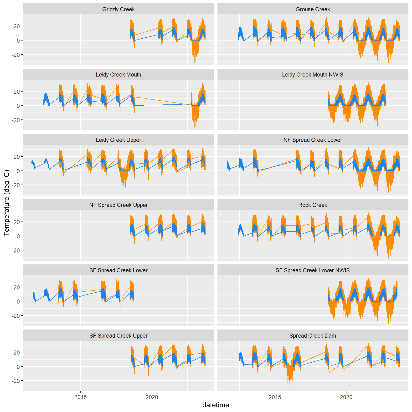
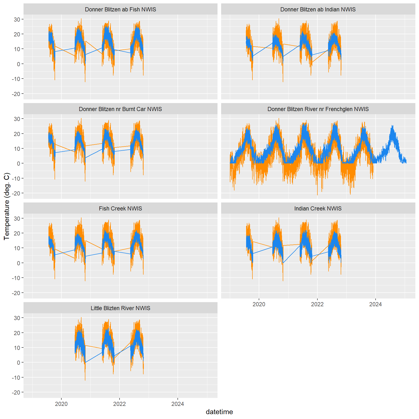
Plot predicted air and stream temperature (orange and blue lines, respectively) over observed air and stream temperature (orange and blue points, respectively).

dat2 %>% 
  select(site_name, datetime, airTemperature, waterTemperature) %>% 
  filter(site_name == focal_site) %>% 
  left_join(preds) %>% 
  filter(site_name == focal_site, rSquared_air >= 0.7 & rSquared_water >= 0.7) %>% 
  select(-c(site_name, rSquared_air, rSquared_water)) %>% 
  mutate(datetime = datetime) %>% # need to fudge datetime b/c dyGraphs converts to local time zone
  dygraph(main = focal_site) %>% dyRangeSelector() %>% 
  #dyAxis("y", label = "Water temp.") %>% 
  #dyAxis("y2", label = "Air temp.") %>% 
  dySeries("waterTemperature", axis = "y", label = "Obs. water temp.", drawPoints = TRUE, strokeWidth = 0, pointSize = 3, color = "dodgerblue") %>% 
  dySeries("airTemperature", axis = "y", label = "Obs. air temp.", drawPoints = TRUE, strokeWidth = 0, pointSize = 3, color = "darkorange")  %>% 
  dySeries("predTemp_water", axis = "y", label = "Pred. water temp.", color = "dodgerblue") %>% 
  dySeries("predTemp_air", axis = "y", label = "Pred. air temp.", color = "darkorange")

7.4.2 All sites

Define subbasins

mysubbasins <- c("West Brook", "Paine Run", "Staunton River", "Big Creek", "Coal Creek", "McGee Creek", "Shields River", "Snake River", "Donner Blitzen", "Duck Creek")

7.4.2.1 Amplitude ratio

Temporal patterns

myplots <- list()
for (i in 1:length(mysubbasins)) {
  mysites <- unlist(siteinfo2 %>% filter(site_name %in% unique(pasta_derived$site_name)) %>% filter(subbasin == mysubbasins[i]) %>% arrange(desc(area_sqmi)) %>% select(site_name))
  myplots[[i]] <- pasta_derived %>% 
    filter(site_name %in% mysites, rSquared_air >= 0.7 & rSquared_water >= 0.7) %>% 
    mutate(year = factor(year), site_name = factor(site_name, levels = mysites)) %>% 
    ggplot(aes(x = yday, y = amplitudeRatio, color = year)) + 
    geom_point(alpha = 0.2) + 
    geom_smooth(se = FALSE) + #geom_smooth(method = "lm", formula = y ~ poly(x, 2)) + 
    ggtitle(mysubbasins[i]) + ylim(0,1) + 
    facet_wrap(~site_name, ncol = 3)
}

West Brook

myplots[[1]]

Paine Run

myplots[[2]]

Staunton River

myplots[[3]]

Big Creek

myplots[[4]]

Coal Creek

myplots[[5]]

McGee Creek

myplots[[6]]

Shields River

myplots[[7]]

Snake River

myplots[[8]]

Donner Blitzen

myplots[[9]]

Duck Creek

myplots[[10]]

By Flow

myplots <- list()
for (i in 1:length(mysubbasins)) {
  mysites <- unlist(siteinfo2 %>% filter(site_name %in% unique(pasta_derived$site_name)) %>% filter(subbasin == mysubbasins[i]) %>% arrange(desc(area_sqmi)) %>% select(site_name))
  myplots[[i]] <- pasta_derived %>% 
    filter(site_name %in% mysites, rSquared_air >= 0.7 & rSquared_water >= 0.7) %>% 
    mutate(year = factor(year), site_name = factor(site_name, levels = mysites)) %>% 
    ggplot(aes(x = z_flow, y = amplitudeRatio, color = year)) + 
    geom_point(alpha = 0.2) + 
    geom_smooth(se = FALSE) + #geom_smooth(method = "lm", formula = y ~ poly(x, 2)) + 
    ggtitle(mysubbasins[i]) + ylim(0,1) + 
    facet_wrap(~site_name, ncol = 3, scales = "free_x")
}

West Brook

myplots[[1]]

Paine Run

myplots[[2]]

Staunton River

myplots[[3]]

Big Creek

myplots[[4]]

Coal Creek

myplots[[5]]

McGee Creek

myplots[[6]]

Shields River

myplots[[7]]

Snake River

myplots[[8]]

Donner Blitzen

myplots[[9]]

Duck Creek

myplots[[10]]

7.4.2.2 Phase lag

Temporal patterns

myplots <- list()
for (i in 1:length(mysubbasins)) {
  mysites <- unlist(siteinfo2 %>% filter(site_name %in% unique(pasta_derived$site_name)) %>% filter(subbasin == mysubbasins[i]) %>% arrange(desc(area_sqmi)) %>% select(site_name))
  myplots[[i]] <- pasta_derived %>% 
    filter(site_name %in% mysites, rSquared_air >= 0.7 & rSquared_water >= 0.7) %>% 
    mutate(year = factor(year), site_name = factor(site_name, levels = mysites)) %>% 
    ggplot(aes(x = yday, y = phaseLag, color = year)) + 
    geom_point(alpha = 0.2) + 
    geom_smooth(se = FALSE) + #geom_smooth(method = "lm", formula = y ~ poly(x, 2)) + 
    ggtitle(mysubbasins[i]) + #ylim(0,1) + 
    geom_abline(slope = 0, intercept = 0, linetype = "dashed") +
    facet_wrap(~site_name, ncol = 3)
}

West Brook

myplots[[1]]

Paine Run

myplots[[2]]

Staunton River

myplots[[3]]

Big Creek

myplots[[4]]

Coal Creek

myplots[[5]]

McGee Creek

myplots[[6]]

Shields River

myplots[[7]]

Snake River

myplots[[8]]

Donner Blitzen

myplots[[9]]

Duck Creek

myplots[[10]]

By Flow

myplots <- list()
for (i in 1:length(mysubbasins)) {
  mysites <- unlist(siteinfo2 %>% filter(site_name %in% unique(pasta_derived$site_name)) %>% filter(subbasin == mysubbasins[i]) %>% arrange(desc(area_sqmi)) %>% select(site_name))
  myplots[[i]] <- pasta_derived %>% 
    filter(site_name %in% mysites, rSquared_air >= 0.7 & rSquared_water >= 0.7) %>% 
    mutate(year = factor(year), site_name = factor(site_name, levels = mysites)) %>% 
    ggplot(aes(x = z_flow, y = phaseLag, color = year)) + 
    geom_point(alpha = 0.2) + 
    geom_smooth(se = FALSE) + #geom_smooth(method = "lm", formula = y ~ poly(x, 2)) + 
    ggtitle(mysubbasins[i]) + #ylim(0,1) + 
    geom_abline(slope = 0, intercept = 0, linetype = "dashed") +
    facet_wrap(~site_name, ncol = 3, scales = "free_x")
}

West Brook

myplots[[1]]

Paine Run

myplots[[2]]

Staunton River

myplots[[3]]

Big Creek

myplots[[4]]

Coal Creek

myplots[[5]]

McGee Creek

myplots[[6]]

Shields River

myplots[[7]]

Snake River

myplots[[8]]

Donner Blitzen

myplots[[9]]

Duck Creek

myplots[[10]]

7.4.2.3 Mean ratio

Temporal patterns

myplots <- list()
for (i in 1:length(mysubbasins)) {
  mysites <- unlist(siteinfo2 %>% filter(site_name %in% unique(pasta_derived$site_name)) %>% filter(subbasin == mysubbasins[i]) %>% arrange(desc(area_sqmi)) %>% select(site_name))
  myplots[[i]] <- pasta_derived %>% 
    filter(site_name %in% mysites, rSquared_air >= 0.7 & rSquared_water >= 0.7, meanRatio >=0, meanRatio <= 2) %>% 
    mutate(year = factor(year), site_name = factor(site_name, levels = mysites)) %>% 
    ggplot(aes(x = yday, y = meanRatio, color = year)) + 
    geom_point(alpha = 0.2) + 
    geom_smooth(se = FALSE) + #geom_smooth(method = "lm", formula = y ~ poly(x, 2)) + 
    ggtitle(mysubbasins[i]) + #ylim(0,1) + 
    facet_wrap(~site_name, ncol = 3)
}

West Brook

myplots[[1]]

Paine Run

myplots[[2]]

Staunton River

myplots[[3]]

Big Creek

myplots[[4]]

Coal Creek

myplots[[5]]

McGee Creek

myplots[[6]]

Shields River

myplots[[7]]

Snake River

myplots[[8]]

Donner Blitzen

myplots[[9]]

Duck Creek

myplots[[10]]

By Flow

myplots <- list()
for (i in 1:length(mysubbasins)) {
  mysites <- unlist(siteinfo2 %>% filter(site_name %in% unique(pasta_derived$site_name)) %>% filter(subbasin == mysubbasins[i]) %>% arrange(desc(area_sqmi)) %>% select(site_name))
  myplots[[i]] <- pasta_derived %>% 
    filter(site_name %in% mysites, rSquared_air >= 0.7 & rSquared_water >= 0.7, meanRatio >=0, meanRatio <= 2) %>% 
    mutate(year = factor(year), site_name = factor(site_name, levels = mysites)) %>% 
    ggplot(aes(x = z_flow, y = meanRatio, color = year)) + 
    geom_point(alpha = 0.2) + 
    geom_smooth(se = FALSE) + #geom_smooth(method = "lm", formula = y ~ poly(x, 2)) + 
    ggtitle(mysubbasins[i]) + #ylim(0,1) + 
    facet_wrap(~site_name, ncol = 3, scales = "free_x")
}

West Brook

myplots[[1]]

Paine Run

myplots[[2]]

Staunton River

myplots[[3]]

Big Creek

myplots[[4]]

Coal Creek

myplots[[5]]

McGee Creek

myplots[[6]]

Shields River

myplots[[7]]

Snake River

myplots[[8]]

Donner Blitzen

myplots[[9]]

Duck Creek

myplots[[10]]

7.4.2.4 Pl-Ar Correlation

myplots <- list()
for (i in 1:length(mysubbasins)) {
  mysites <- unlist(siteinfo2 %>% filter(site_name %in% unique(pasta_derived$site_name)) %>% filter(subbasin == mysubbasins[i]) %>% arrange(desc(area_sqmi)) %>% select(site_name))
  myplots[[i]] <- pasta_derived %>% 
    filter(site_name %in% mysites, rSquared_air >= 0.7 & rSquared_water >= 0.7, phaseLag >= -5, phaseLag <= 10, amplitudeRatio >= 0, amplitudeRatio <= 1) %>% 
    mutate(year = factor(year), site_name = factor(site_name, levels = mysites)) %>% 
    ggplot(aes(x = amplitudeRatio, y = phaseLag, color = z_flow)) + 
    geom_point(alpha = 0.5) + 
    #geom_smooth(se = FALSE) + #geom_smooth(method = "lm", formula = y ~ poly(x, 2)) + 
    ggtitle(mysubbasins[i]) + #ylim(0,1) + 
    facet_wrap(~site_name, ncol = 3)
}

West Brook

myplots[[1]]

Paine Run

myplots[[2]]

Staunton River

myplots[[3]]

Big Creek

myplots[[4]]

Coal Creek

myplots[[5]]

McGee Creek

myplots[[6]]

Shields River

myplots[[7]]

Snake River

myplots[[8]]

Donner Blitzen

myplots[[9]]

Duck Creek

myplots[[10]]

7.5 Summarize output

7.5.1 Rolling mean

7.5.1.1 Summarize

Summarize PASTA output as 7-day rolling means for use in the Wedge Model and elsewhere, per Rey et al. (2024)

Interpolate short gaps and calulate 7-day rolling mean

# Drop poor fits then fill missing dates
pasta_derived_filled <- fill_missing_dates(pasta_derived %>% filter(rSquared_air >= 0.7 & rSquared_water >= 0.7), dates = date, groups = site_name) #%>% group_by(site_name) %>% arrange(site_name, date) 

# get rid of crazy mean ratio values
pasta_derived_filled <- pasta_derived_filled %>%
  mutate(meanRatio = ifelse(meanRatio < 0, NA,
                            ifelse(meanRatio > 2, NA, meanRatio)))

# Interpolate short gaps (<=3 days) and calculate 7-day rolling mean as in Rey et al. (2024)
datalist <- list()
mysites <- unique(pasta_derived_filled$site_name)
for (i in 1:length(mysites)) { 
  datalist[[i]] <- pasta_derived_filled %>% 
    filter(site_name == mysites[i]) %>% 
    mutate(amplitudeRatio_fill = na.approx(amplitudeRatio, maxgap = 3, na.rm = FALSE),
           phaseLag_fill = na.approx(phaseLag, maxgap = 3, na.rm = FALSE),
           meanRatio_fill = na.approx(meanRatio, maxgap = 3, na.rm = FALSE)) %>%
    mutate(amplitudeRatio_fill_roll7 = rollapply(amplitudeRatio_fill, FUN = mean, width = 7, align = "center", fill = NA),
           phaseLag_fill_roll7 = rollapply(phaseLag_fill, FUN = mean, width = 7, align = "center", fill = NA),
           meanRatio_fill_roll7 = rollapply(meanRatio_fill, FUN = mean, width = 7, align = "center", fill = NA))
}
pasta_derived_filled <- do.call(rbind, datalist)

Write to file

write_csv(pasta_derived_filled, "C:/Users/jbaldock/OneDrive - DOI/Documents/USGS/EcoDrought/EcoDrought Working/EcoDrought-Analysis/Covariates/pasta_derived_parameters_7daymean.csv")

Set focal site

focal_site <- "McGeeCreekUpper"
print(focal_site)

[1] "McGeeCreekUpper"

View focal data

pasta_derived_filled %>% 
  filter(site_name == focal_site, rSquared_air >= 0.7 & rSquared_water >= 0.7) 

# A tibble: 974 × 24
   site_name      date        year  yday amplitude_air amplitude_water phase_air
   <chr>          <date>     <dbl> <dbl>         <dbl>           <dbl>     <dbl>
 1 McGeeCreekUpp… 2017-08-02  2017   214          4.86           1.08       6.46
 2 McGeeCreekUpp… 2017-08-03  2017   215          9.33           1.26       8.12
 3 McGeeCreekUpp… 2017-08-04  2017   216          9.39           1.14       8.31
 4 McGeeCreekUpp… 2017-08-05  2017   217          4.11           0.945      7.47
 5 McGeeCreekUpp… 2017-08-06  2017   218          9.13           1.10       8.40
 6 McGeeCreekUpp… 2017-08-07  2017   219         10.3            1.14       8.43
 7 McGeeCreekUpp… 2017-08-08  2017   220          6.72           0.913      6.70
 8 McGeeCreekUpp… 2017-08-09  2017   221          9.14           1.05       7.57
 9 McGeeCreekUpp… 2017-08-10  2017   222          8.98           1.02       7.84
10 McGeeCreekUpp… 2017-08-11  2017   223          9.57           1.01       7.96
# ℹ 964 more rows
# ℹ 17 more variables: phase_water <dbl>, mean_air <dbl>, mean_water <dbl>,
#   rSquared_air <dbl>, rSquared_water <dbl>, amplitudeRatio <dbl>,
#   phaseLag <dbl>, meanRatio <dbl>, meanOffset <dbl>, flow <dbl>,
#   z_flow <dbl>, amplitudeRatio_fill <dbl>, phaseLag_fill <dbl>,
#   meanRatio_fill <dbl>, amplitudeRatio_fill_roll7 <dbl>,
#   phaseLag_fill_roll7 <dbl>, meanRatio_fill_roll7 <dbl>

Amplitude Ratio

pasta_derived_filled %>% 
  filter(site_name == focal_site, rSquared_air >= 0.7 & rSquared_water >= 0.7) %>% 
  ggplot() + 
  geom_point(aes(x = yday, y = amplitudeRatio), color = "black") + ggtitle(focal_site) + 
  geom_point(aes(x = yday, y = amplitudeRatio_fill_roll7), color = "red") + ggtitle(focal_site) + 
  #geom_smooth(method = "lm", formula = y ~ poly(x, 2)) + 
  facet_wrap(~year)

Phase Lag

pasta_derived_filled %>% 
  filter(site_name == focal_site, rSquared_air >= 0.7 & rSquared_water >= 0.7) %>% 
  ggplot() + 
  geom_point(aes(x = yday, y = phaseLag), color = "black") + ggtitle(focal_site) + 
  geom_point(aes(x = yday, y = phaseLag_fill_roll7), color = "red") + ggtitle(focal_site) + 
  #geom_smooth(method = "lm", formula = y ~ poly(x, 2)) + 
  facet_wrap(~year)

Mean Ratio

pasta_derived_filled %>% 
  filter(site_name == focal_site, rSquared_air >= 0.7 & rSquared_water >= 0.7) %>% 
  ggplot() + 
  geom_point(aes(x = yday, y = meanRatio), color = "black") + ggtitle(focal_site) + 
  geom_point(aes(x = yday, y = meanRatio_fill_roll7), color = "red") + ggtitle(focal_site) + 
  #geom_smooth(method = "lm", formula = y ~ poly(x, 2)) + 
  facet_wrap(~year)

7.5.1.2 Calculate Gg difference

Join big G PASTA derived parameters (7-day rolling means) to little g PASTA derived parameters and calculate difference (little - big).

pasta_derived_filled_big <- pasta_derived_filled %>% left_join(siteinfo2 %>% select(site_name, subbasin, designation)) %>% filter(designation == "big") %>% select(-designation)

pasta_derived_filled_little <- pasta_derived_filled %>% left_join(siteinfo2 %>% select(site_name, subbasin, designation)) %>% filter(designation == "little") %>% select(-designation)

pasta_derived_filled_join <- pasta_derived_filled_little %>% 
  select(site_name, subbasin, date, rSquared_air, rSquared_water, amplitudeRatio_fill_roll7, phaseLag_fill_roll7, meanRatio_fill_roll7) %>% 
  rename(site_name_little = site_name, rSquared_air_little = rSquared_air, rSquared_water_little = rSquared_water, amplitudeRatio_fill_roll7_little = amplitudeRatio_fill_roll7, phaseLag_fill_roll7_little = phaseLag_fill_roll7, meanRatio_fill_roll7_little = meanRatio_fill_roll7) %>% 
  left_join(pasta_derived_filled_big %>% 
  select(site_name, subbasin, date, rSquared_air, rSquared_water, amplitudeRatio_fill_roll7, phaseLag_fill_roll7, meanRatio_fill_roll7) %>% 
  rename(site_name_big = site_name, rSquared_air_big = rSquared_air, rSquared_water_big = rSquared_water, amplitudeRatio_fill_roll7_big = amplitudeRatio_fill_roll7, phaseLag_fill_roll7_big = phaseLag_fill_roll7, meanRatio_fill_roll7_big = meanRatio_fill_roll7)) %>% 
  filter(rSquared_air_little >= 0.7, rSquared_water_little >= 0.7, rSquared_air_big >= 0.7, rSquared_water_big >= 0.7) %>%
  mutate(amplitudeRatio_diff = amplitudeRatio_fill_roll7_little - amplitudeRatio_fill_roll7_big,
         phaseLag_diff = phaseLag_fill_roll7_little - phaseLag_fill_roll7_big,
         meanRatio_diff = meanRatio_fill_roll7_little - meanRatio_fill_roll7_big,
         yday = yday(date),
         year = year(date))

Write to file

write_csv(pasta_derived_filled_join, "C:/Users/jbaldock/OneDrive - DOI/Documents/USGS/EcoDrought/EcoDrought Working/EcoDrought-Analysis/Covariates/pasta_derived_parameters_7daymean_gGdiff.csv")

Amplitude ratio

myplots <- list()
for (i in 1:length(mysubbasins)) {
  mysites <- unlist(siteinfo2 %>% filter(site_name %in% unique(pasta_derived$site_name)) %>% filter(subbasin == mysubbasins[i], designation == "little") %>% arrange(desc(area_sqmi)) %>% select(site_name))
  myplots[[i]] <- pasta_derived_filled_join %>% 
    filter(site_name_little %in% mysites) %>% 
    mutate(year = factor(year), site_name = factor(site_name_little, levels = mysites)) %>% 
    ggplot(aes(x = yday, y = amplitudeRatio_diff, color = year)) + 
    geom_point(alpha = 0.5) + 
    geom_abline(slope = 0, intercept = 0, linetype = "dashed") +
    ggtitle(mysubbasins[i]) + #ylim(0,1) + 
    facet_wrap(~site_name_little, ncol = 3)
}

West Brook

myplots[[1]]

Paine Run

myplots[[2]]

Staunton River

myplots[[3]]

Big Creek

myplots[[4]]

Coal Creek

myplots[[5]]

McGee Creek

myplots[[6]]

Shields River

myplots[[7]]

Snake River

myplots[[8]]

Donner Blitzen

myplots[[9]]

Duck Creek

myplots[[10]]

Phase lag

myplots <- list()
for (i in 1:length(mysubbasins)) {
  mysites <- unlist(siteinfo2 %>% filter(site_name %in% unique(pasta_derived$site_name)) %>% filter(subbasin == mysubbasins[i], designation == "little") %>% arrange(desc(area_sqmi)) %>% select(site_name))
  myplots[[i]] <- pasta_derived_filled_join %>% 
    filter(site_name_little %in% mysites) %>% 
    mutate(year = factor(year), site_name = factor(site_name_little, levels = mysites)) %>% 
    ggplot(aes(x = yday, y = phaseLag_diff, color = year)) + 
    geom_point(alpha = 0.5) + 
    geom_abline(slope = 0, intercept = 0, linetype = "dashed") +
    ggtitle(mysubbasins[i]) + #ylim(0,1) + 
    facet_wrap(~site_name_little, ncol = 3)
}

West Brook

myplots[[1]]

Paine Run

myplots[[2]]

Staunton River

myplots[[3]]

Big Creek

myplots[[4]]

Coal Creek

myplots[[5]]

McGee Creek

myplots[[6]]

Shields River

myplots[[7]]

Snake River

myplots[[8]]

Donner Blitzen

myplots[[9]]

Duck Creek

myplots[[10]]

Mean ratio

myplots <- list()
for (i in 1:length(mysubbasins)) {
  mysites <- unlist(siteinfo2 %>% filter(site_name %in% unique(pasta_derived$site_name)) %>% filter(subbasin == mysubbasins[i], designation == "little") %>% arrange(desc(area_sqmi)) %>% select(site_name))
  myplots[[i]] <- pasta_derived_filled_join %>% 
    filter(site_name_little %in% mysites) %>% 
    mutate(year = factor(year), site_name = factor(site_name_little, levels = mysites)) %>% 
    ggplot(aes(x = yday, y = meanRatio_diff, color = year)) + 
    geom_point(alpha = 0.5) + 
    geom_abline(slope = 0, intercept = 0, linetype = "dashed") +
    ggtitle(mysubbasins[i]) + #ylim(0,1) + 
    facet_wrap(~site_name_little, ncol = 3)
}

West Brook

myplots[[1]]

Paine Run

myplots[[2]]

Staunton River

myplots[[3]]

Big Creek

myplots[[4]]

Coal Creek

myplots[[5]]

McGee Creek

myplots[[6]]

Shields River

myplots[[7]]

Snake River

myplots[[8]]

Donner Blitzen

myplots[[9]]

Duck Creek

myplots[[10]]

7.5.2 August mean

Summarize gG differenced PASTA output as site-level August means, across all years.

pasta_derived_august <- pasta_derived_filled_join %>% 
  mutate(month = month(date)) %>% 
  filter(month == 8, 
         rSquared_air_little >= 0.7, rSquared_water_little >= 0.7, 
         rSquared_air_big >= 0.7, rSquared_water_big >= 0.7) %>% 
  group_by(site_name_little) %>% 
  summarize(amplitudeRatio_little_AugMean = mean(amplitudeRatio_fill_roll7_little, na.rm = TRUE),
            phaseLag_little_AugMean = mean(phaseLag_fill_roll7_little, na.rm = TRUE),
            meanRatio_little_AugMean = mean(meanRatio_fill_roll7_little, na.rm = TRUE),
            amplitudeRatio_big_AugMean = mean(amplitudeRatio_fill_roll7_big, na.rm = TRUE),
            phaseLag_big_AugMean = mean(phaseLag_fill_roll7_big, na.rm = TRUE),
            meanRatio_big_AugMean = mean(meanRatio_fill_roll7_big, na.rm = TRUE),
            amplitudeRatio_diff_AugMean = mean(amplitudeRatio_diff, na.rm = TRUE),
            phaseLag_diff_AugMean = mean(phaseLag_diff, na.rm = TRUE),
            meanRatio_diff_AugMean = mean(meanRatio_diff, na.rm = TRUE))
head(pasta_derived_august)

# A tibble: 6 × 10
  site_name_little    amplitudeRatio_little_AugMean phaseLag_little_AugMean
  <chr>                                       <dbl>                   <dbl>
1 Avery Brook                                 0.221                    2.19
2 BigCreekMiddle                              0.364                    1.47
3 BigCreekUpper                               0.152                    2.38
4 Buck Creek                                  0.379                    1.17
5 CoalCreekHeadwaters                         0.193                    2.30
6 CoalCreekMiddle                             0.189                    1.62
# ℹ 7 more variables: meanRatio_little_AugMean <dbl>,
#   amplitudeRatio_big_AugMean <dbl>, phaseLag_big_AugMean <dbl>,
#   meanRatio_big_AugMean <dbl>, amplitudeRatio_diff_AugMean <dbl>,
#   phaseLag_diff_AugMean <dbl>, meanRatio_diff_AugMean <dbl>

Write to file

write_csv(pasta_derived_august, "C:/Users/jbaldock/OneDrive - DOI/Documents/USGS/EcoDrought/EcoDrought Working/EcoDrought-Analysis/Covariates/pasta_derived_parameters_AugustDiff.csv")