Code
siteinfo <- read_csv("C:/Users/jbaldock/OneDrive - DOI/Documents/USGS/EcoDrought/EcoDrought Working/Data/EcoDrought_SiteInformation.csv")
datatable(siteinfo)This section contains the code for reproducing the analysis described in Baldock et al., Headwater streamflow variability is amplified by drought. This page/chapter organizes all the streamflow data, previously collated into a single file (see Chapter 2 - Collate Data), and conducts the hydroclimate analysis (data pulled from Knoben et al. 2018, Water Resources Research).
Significance: Headwater streams account for a majority of river networks worldwide and have a disproportionately large influence on the functioning of aquatic ecosystems. Headwater streams also support critical habitat for many species, including cold-water fishes, many of which are declining or at risk of extinction.
Problem: Headwater streams are largely underrepresented in streamflow monitoring networks, which place greater emphasis on mainstem rivers. As a result, less is known about how headwaters respond to changing water availability. Headwater streams therefore represent a blind spot in understanding flow regime variability and assessing the vulnerability of cold-water fish to changing climatic conditions, including the increasing frequency and severity of drought.
Questions:
Approach:
View site information
siteinfo <- read_csv("C:/Users/jbaldock/OneDrive - DOI/Documents/USGS/EcoDrought/EcoDrought Working/Data/EcoDrought_SiteInformation.csv")
datatable(siteinfo)Map sites
siteinfo_sp <- st_as_sf(siteinfo, coords = c("long", "lat"), crs = 4326)
mapview(siteinfo_sp, zcol = "designation")# Write shapefile of focal sites for external mapping
focalsites <- siteinfo_sp %>%
filter(site_name %in% c("West Brook NWIS", "West Brook Lower", "Mitchell Brook", "Jimmy Brook", "Obear Brook Lower", "West Brook Upper", "West Brook Reservoir", "Sanderson Brook", "Avery Brook", "West Whately Brook", "South River Conway NWIS",
"Paine Run 10", "Paine Run 08", "Paine Run 07", "Paine Run 06", "Paine Run 02", "Paine Run 01", "South River Harriston NWIS",
"Staunton River 10", "Staunton River 09", "Staunton River 07", "Staunton River 06", "Staunton River 03", "Staunton River 02", "Rapidan River NWIS",
"BigCreekLower", "LangfordCreekLower", "LangfordCreekUpper", "Big Creek NWIS", "BigCreekUpper", "HallowattCreekLower", "NicolaCreek", "WernerCreek", "Hallowat Creek NWIS", "CoalCreekLower", "CycloneCreekLower", "CycloneCreekMiddle", "CycloneCreekUpper", "CoalCreekMiddle", "CoalCreekNorth", "CoalCreekHeadwaters", "McGeeCreekLower", "McGeeCreekTrib", "McGeeCreekUpper", "North Fork Flathead River NWIS",
"Shields River Valley Ranch", "Deep Creek", "Crandall Creek", "Buck Creek", "Dugout Creek", "Shields River ab Dugout", "Lodgepole Creek", "EF Duck Creek be HF", "EF Duck Creek ab HF", "Henrys Fork", "Yellowstone River Livingston NWIS",
"Spread Creek Dam", "Rock Creek", "NF Spread Creek Lower", "NF Spread Creek Upper", "Grizzly Creek", "SF Spread Creek Lower", "Grouse Creek", "SF Spread Creek Upper", "Leidy Creek Mouth", "Pacific Creek at Moran NWIS",
"Fish Creek NWIS", "Donner Blitzen ab Fish NWIS", "Donner Blitzen nr Burnt Car NWIS", "Donner Blitzen ab Indian NWIS", "Donner Blitzen River nr Frenchglen NWIS")) %>%
mutate(designation = ifelse(designation == "big", "big", "little"))
mapview(focalsites, zcol = "designation")# st_write(focalsites, "C:/Users/jbaldock/OneDrive - DOI/Documents/USGS/EcoDrought/EcoDrought Working/Study area maps/sites/focalsites.shp")Little g daily data
# flow/yield (and temp) data
dat <- read_csv("C:/Users/jbaldock/OneDrive - DOI/Documents/USGS/EcoDrought/EcoDrought Working/Data/EcoDrought_FlowTempData_DailyWeekly.csv") %>%
mutate(site_name = dplyr::recode(site_name, "Leidy Creek Mouth NWIS" = "Leidy Creek Mouth", "SF Spread Creek Lower NWIS" = "SF Spread Creek Lower", "Dugout Creek NWIS" = "Dugout Creek", "Shields River ab Smith NWIS" = "Shields River Valley Ranch")) %>%
filter(!site_name %in% c("Avery Brook NWIS", "West Brook 0", "BigCreekMiddle", # drop co-located sites
"South River Conway NWIS", "North Fork Flathead River NWIS", # drop big Gs
"Pacific Creek at Moran NWIS", "Shields River nr Livingston NWIS", # drop big Gs
"Donner Blitzen River nr Frenchglen NWIS", # drop big Gs
"WoundedBuckCreek")) %>% # drop little g outside of focal basin
group_by(site_name, basin, subbasin, region, date) %>%
summarize(flow_mean = mean(flow_mean),
tempc_mean = mean(tempc_mean),
Yield_mm = mean(Yield_mm),
Yield_filled_mm = mean(Yield_filled_mm)) %>%
ungroup()
# add water/climate year variables and fill missing dates
dat <- fill_missing_dates(dat, dates = date, groups = site_name)
dat <- add_date_variables(dat, dates = date, water_year_start = 10)Clean and bind little g data (for each basin, restrict to time period for which data quality/availability is ~consistent)
dat_clean <- bind_rows(
dat %>% filter(site_name %in% unlist(siteinfo %>% filter(subbasin == "West Brook") %>% select(site_name)), year(date) >= 2020, date <= date("2025-01-03")) %>%
mutate(Yield_filled_mm = ifelse(site_name == "West Brook Upper" & date > date("2024-10-06"), NA, Yield_filled_mm)) %>%
mutate(Yield_filled_mm = ifelse(site_name == "Mitchell Brook" & date > date("2021-02-28") & date < date("2021-03-26"), NA, Yield_filled_mm)) %>%
mutate(Yield_filled_mm = ifelse(site_name == "Mitchell Brook" & date > date("2021-11-01") & date < date("2022-05-01"), NA, Yield_filled_mm)) %>%
mutate(Yield_filled_mm = ifelse(site_name == "Jimmy Brook" & date > date("2024-12-10"), NA, Yield_filled_mm)) %>%
mutate(subbasin = "West Brook"),
dat %>% filter(site_name %in% unlist(siteinfo %>% filter(subbasin == "Paine Run") %>% select(site_name)), date >= as_date("2018-11-07"), date <= as_date("2023-05-15")) %>% mutate(subbasin = "Paine Run"),
dat %>% filter(site_name %in% unlist(siteinfo %>% filter(subbasin == "Staunton River") %>% select(site_name)), date >= as_date("2018-11-07"), date <= as_date("2022-10-19")) %>% mutate(subbasin = "Staunton River"),
dat %>% filter(site_name %in% c(unlist(siteinfo %>% filter(subbasin == "Big Creek") %>% select(site_name)), "North Fork Flathead River NWIS"), date >= date("2018-08-08"), date <= date("2023-08-03"), site_name != "SkookoleelCreek", Yield_filled_mm > 0) %>% mutate(subbasin = "Big Creek"),
dat %>% filter(site_name %in% c(unlist(siteinfo %>% filter(subbasin == "Coal Creek") %>% select(site_name)), "North Fork Flathead River NWIS"), date >= date("2018-07-29"), date <= date("2023-08-03")) %>% mutate(subbasin = "Coal Creek"),
dat %>% filter(site_name %in% c(unlist(siteinfo %>% filter(subbasin == "McGee Creek") %>% select(site_name)), "North Fork Flathead River NWIS"), date >= date("2017-07-30"), date <= date("2023-12-11")) %>% mutate(subbasin = "McGee Creek"),
dat %>% filter(subbasin == "Snake River", date >= date("2016-04-01"), date <= date("2023-10-03"), site_name != "Leidy Creek Upper") %>% mutate(subbasin = "Snake River"),
dat %>% filter(subbasin == "Shields River", date >= date("2016-04-01"), date <= date("2023-12-31"), site_name != "Brackett Creek") %>%
mutate(logYield = log10(Yield_filled_mm)) %>% mutate(subbasin = "Shields River"),
dat %>% filter(subbasin == "Duck Creek", date >= date("2015-04-01"), date <= date("2023-12-31")) %>% mutate(subbasin = "Duck Creek"),
dat %>% filter(subbasin == "Donner Blitzen", date >= as_date("2019-04-23"), date <= as_date("2022-12-31"), !site_name %in% c("Indian Creek NWIS", "Little Blizten River NWIS")) %>% mutate(subbasin = "Donner Blitzen")
) %>%
filter(Yield_filled_mm > 0) %>%
mutate(logYield = log10(Yield_filled_mm),
designation = "little",
doy_calendar = yday(date)) %>%
select(-Yield_mm) %>%
rename(Yield_mm = Yield_filled_mm)
head(dat_clean)# A tibble: 6 × 16
site_name basin subbasin region date flow_mean tempc_mean Yield_mm
<chr> <chr> <chr> <chr> <date> <dbl> <dbl> <dbl>
1 Avery Brook West Bro… West Br… Mass 2020-01-08 5.96 0.594 1.99
2 Avery Brook West Bro… West Br… Mass 2020-01-09 4.81 0.0336 1.61
3 Avery Brook West Bro… West Br… Mass 2020-01-10 4.88 0.363 1.63
4 Avery Brook West Bro… West Br… Mass 2020-01-11 6.43 1.77 2.15
5 Avery Brook West Bro… West Br… Mass 2020-01-12 21.2 2.81 7.08
6 Avery Brook West Bro… West Br… Mass 2020-01-13 14.3 1.92 4.78
# ℹ 8 more variables: CalendarYear <dbl>, Month <dbl>, MonthName <fct>,
# WaterYear <dbl>, DayofYear <dbl>, logYield <dbl>, designation <chr>,
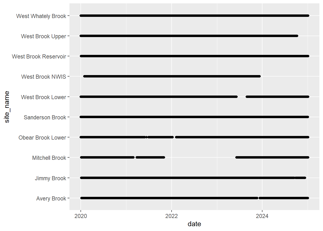
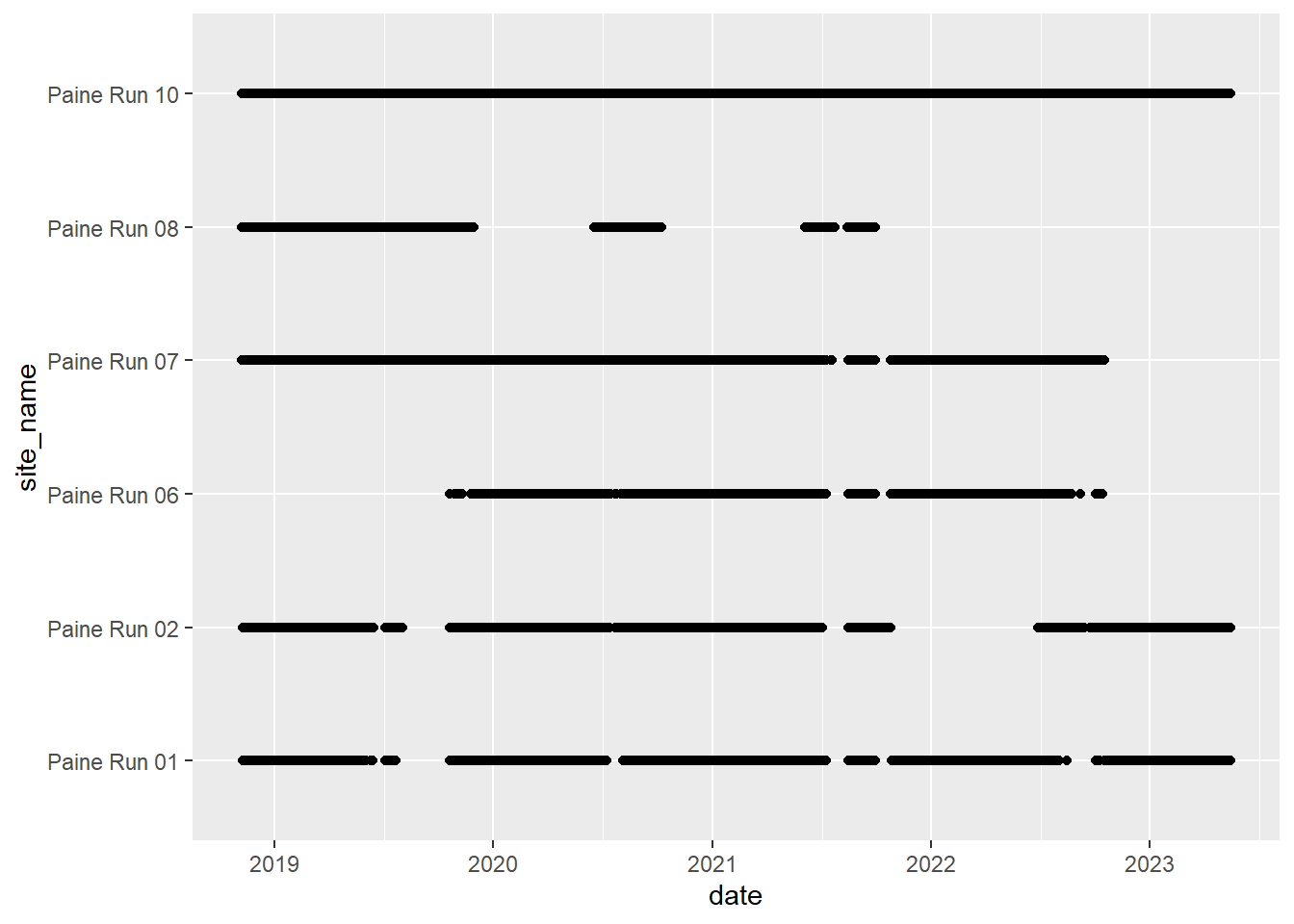
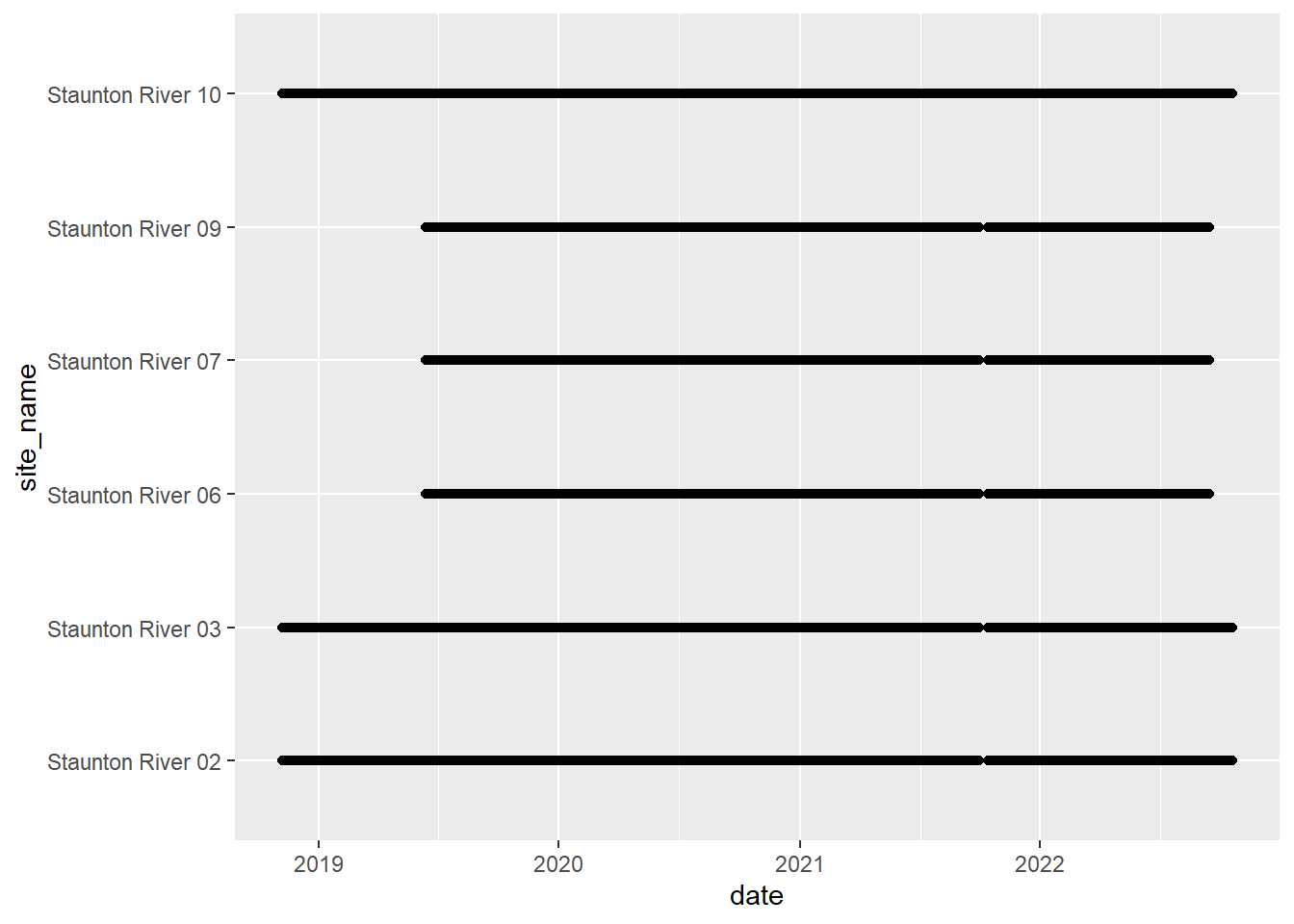
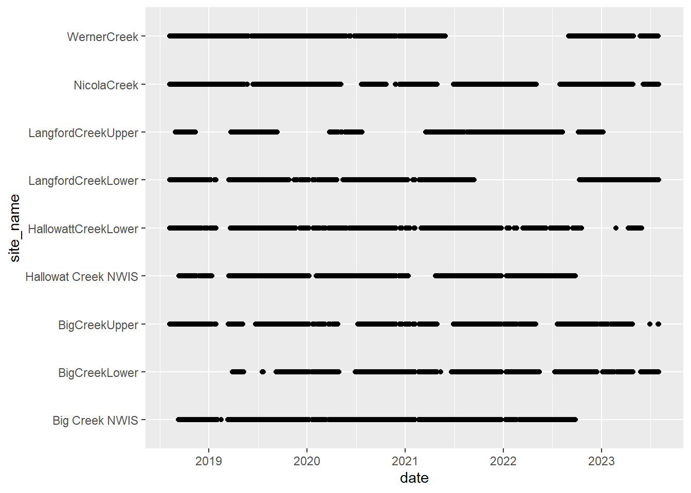
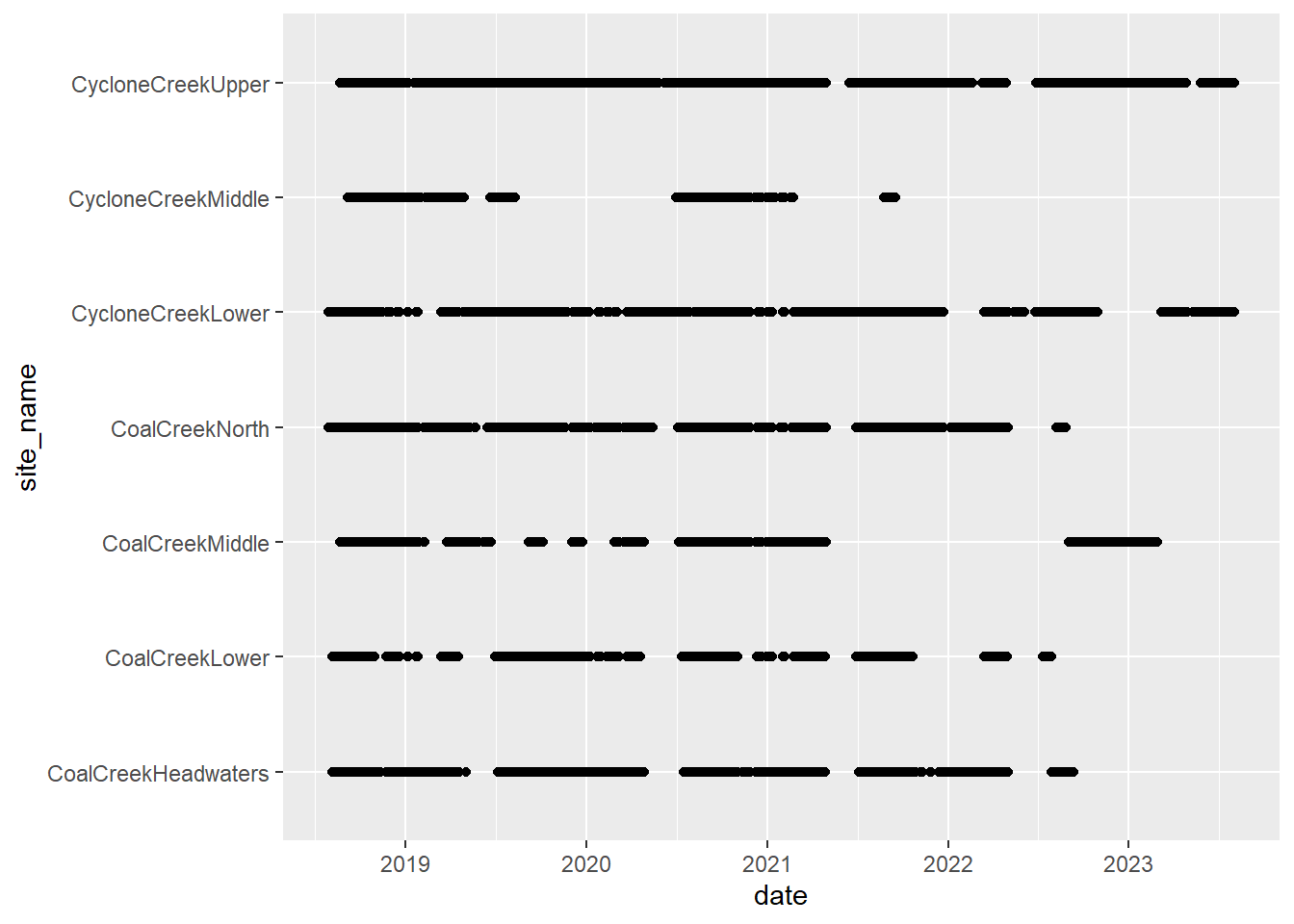
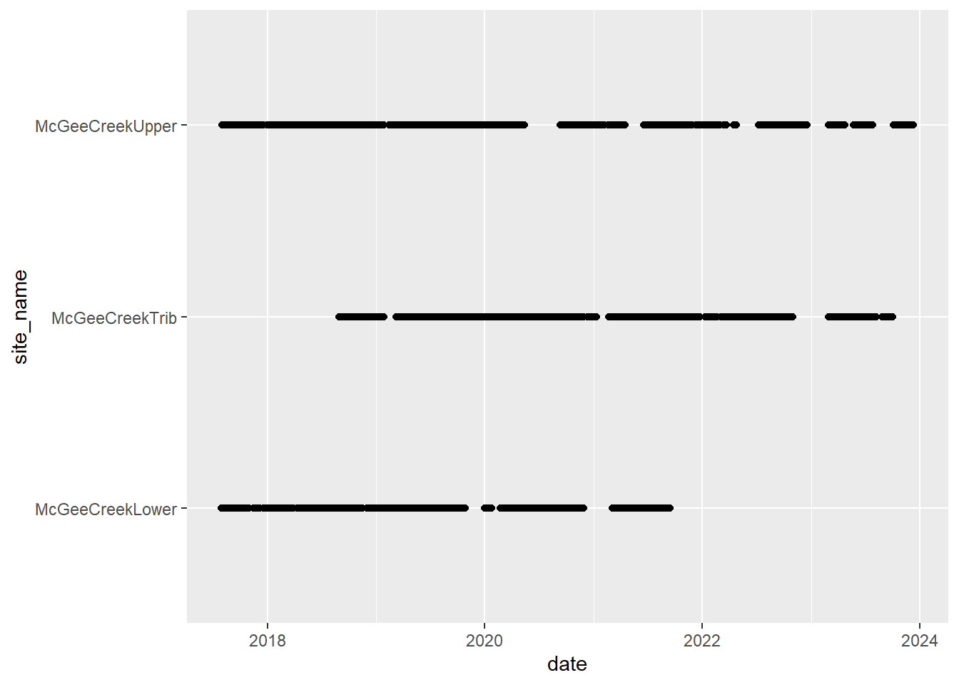
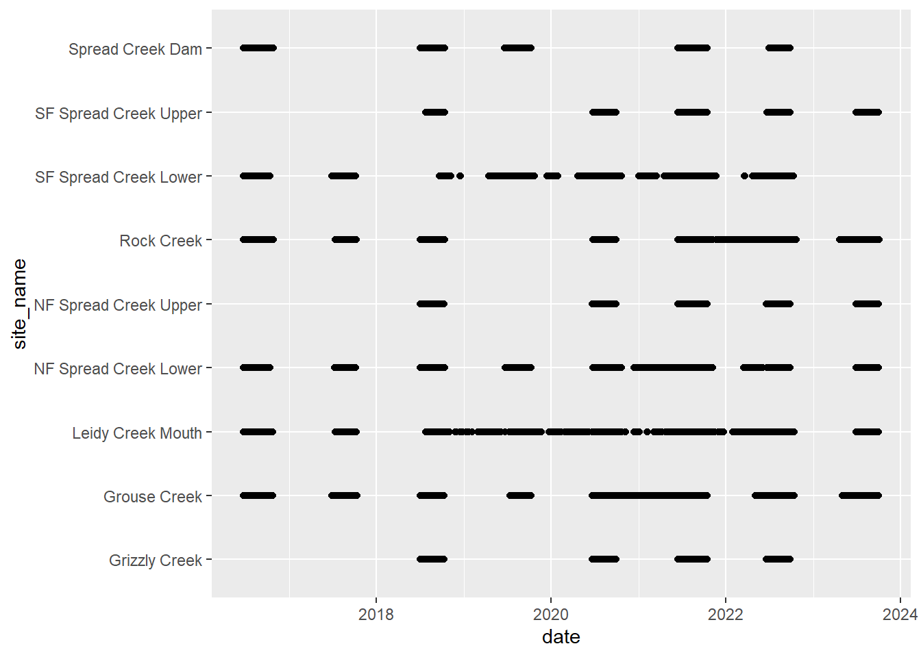
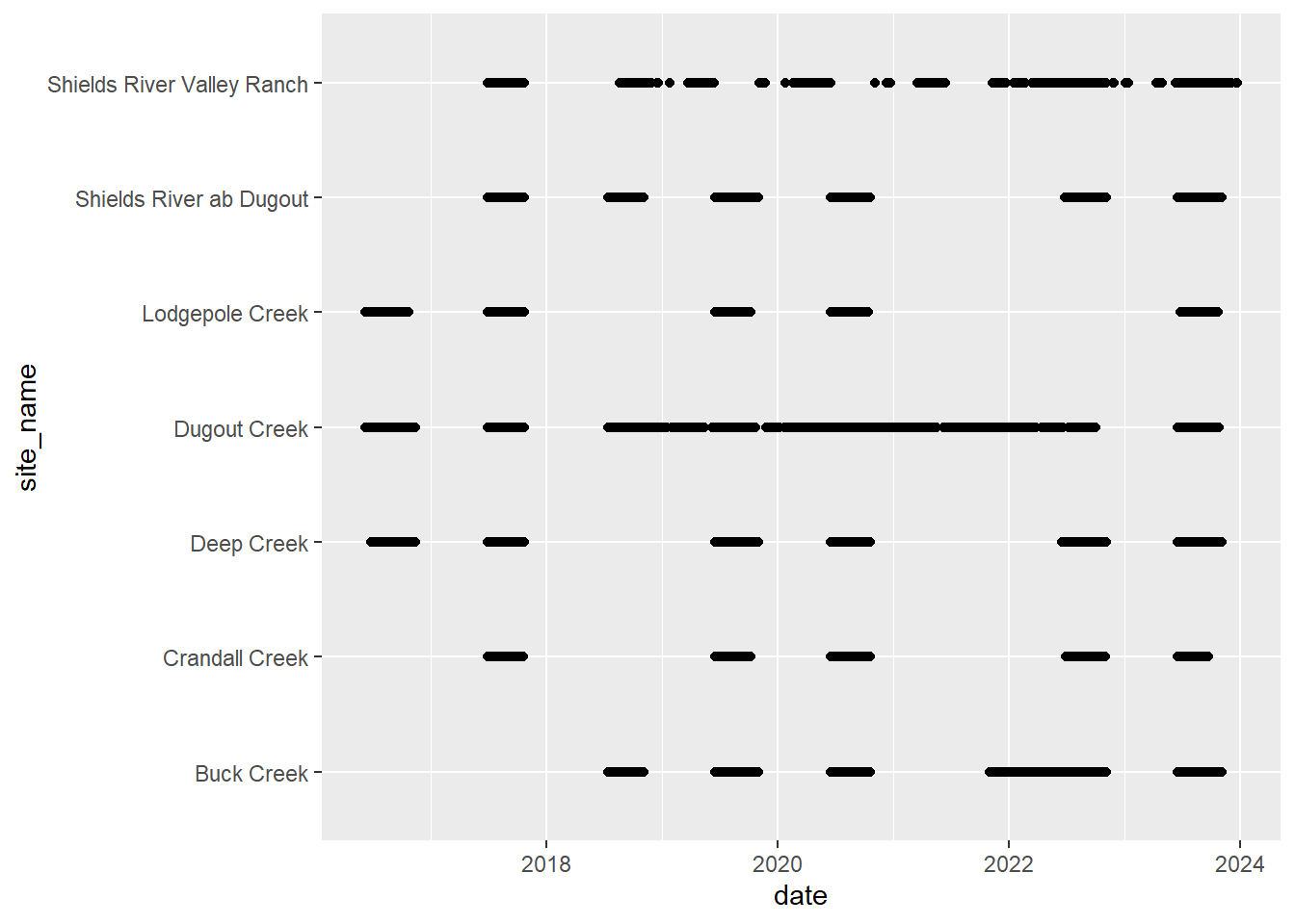
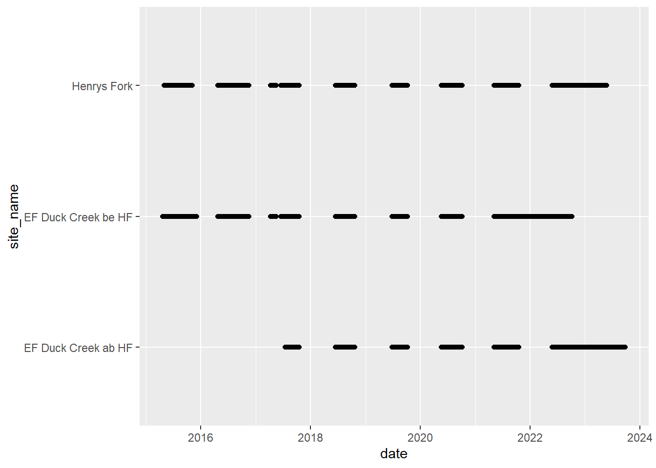
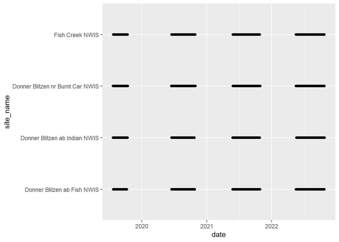
# doy_calendar <dbl>View streamflow data availability by subbasin and site
Write to file
write_csv(dat_clean, "C:/Users/jbaldock/OneDrive - DOI/Documents/USGS/EcoDrought/EcoDrought Working/EcoDrought-Analysis/Qualitative/LittleG_data_clean.csv")p1 <- siteinfo %>%
filter(site_name %in% unique(dat_clean$site_name)) %>%
mutate(area_sqkm = area_sqmi*2.58999,
basin = factor(basin, levels = c("Donner Blitzen", "Snake River", "Flathead", "Shields River",
"Paine Run", "Staunton River", "West Brook"))) %>%
mutate(basin = recode(basin, "Shields River" = "Yellowstone River", "Flathead" = "Flathead River", "Donner Blitzen" = "Donner und Blitzen River")) %>%
ggplot() +
geom_boxplot(aes(y = basin, x = area_sqkm, fill = basin)) + scale_x_log10() +
geom_point(aes(y = basin, x = area_sqkm)) +
theme_bw() + theme(panel.grid = element_blank(), legend.position = "none", axis.text = element_text(color = "black")) +
xlab(expression(paste("Catchment area, km"^2))) + ylab("Basin") +
scale_fill_manual(values = rev(brewer.pal(7, "Set2")[c(1,2,3,5,4,6,7)]))
jpeg("C:/Users/jbaldock/OneDrive - DOI/Documents/USGS/EcoDrought/EcoDrought Working/Presentation figs/CatchmentSize_boxplot.jpg", width = 5, height = 3, units = "in", res = 1000)
p1
dev.off()png
2 Load big/super G data
nwis_daily <- read_csv("C:/Users/jbaldock/OneDrive - DOI/Documents/USGS/EcoDrought/EcoDrought Working/Data/EcoDrought_NWIS_FlowTempData_Raw_Daily.csv") %>%
filter(designation == "big",
year(date) >= 1970,
site_name != "Shields River nr Livingston NWIS") %>%
mutate(flowcfs = ifelse(site_name == "Rapidan River NWIS" & date > date("1995-06-26") & date < date("1995-07-01"), NA, flowcfs),
flow_mean_cms = flowcfs*0.02831683199881,
area_sqkm = area_sqmi*2.58999)
# sites
sites <- unique(nwis_daily$site_name)
# site-specific basin area in square km
basinarea <- nwis_daily %>% filter(!is.na(site_id)) %>% group_by(site_name) %>% summarize(area_sqkm = unique(area_sqkm))
# calculate yield
yield_list <- list()
for (i in 1:length(sites)) {
d <- nwis_daily %>% filter(site_name == sites[i])
ba <- unlist(basinarea %>% filter(site_name == sites[i]) %>% select(area_sqkm))
yield_list[[i]] <- add_daily_yield(data = d, values = flow_mean_cms, basin_area = as.numeric(ba))
}
nwis_daily_wyield <- do.call(rbind, yield_list)
dat_clean_big <- nwis_daily_wyield %>%
select(site_name, basin, subbasin, region, date, Yield_mm, tempc, flowcfs) %>%
mutate(logYield = log10(Yield_mm), doy_calendar = yday(date)) %>%
rename(tempc_mean = tempc, flow_mean = flowcfs)
# add water/climate year variables and fill missing dates
dat_clean_big <- fill_missing_dates(dat_clean_big, dates = date, groups = site_name)
dat_clean_big <- add_date_variables(dat_clean_big, dates = date, water_year_start = 10)
head(dat_clean_big)# A tibble: 6 × 15
site_name basin subbasin region date Yield_mm tempc_mean flow_mean
<chr> <chr> <chr> <chr> <date> <dbl> <dbl> <dbl>
1 South River Co… West… West Br… Mass 1970-01-01 1.81 NA 46
2 South River Co… West… West Br… Mass 1970-01-02 1.69 NA 43
3 South River Co… West… West Br… Mass 1970-01-03 1.61 NA 41
4 South River Co… West… West Br… Mass 1970-01-04 1.53 NA 39
5 South River Co… West… West Br… Mass 1970-01-05 1.49 NA 38
6 South River Co… West… West Br… Mass 1970-01-06 1.49 NA 38
# ℹ 7 more variables: logYield <dbl>, doy_calendar <dbl>, CalendarYear <dbl>,
# Month <dbl>, MonthName <fct>, WaterYear <dbl>, DayofYear <dbl>Write to file
write_csv(dat_clean_big, "C:/Users/jbaldock/OneDrive - DOI/Documents/USGS/EcoDrought/EcoDrought Working/EcoDrought-Analysis/Qualitative/BigG_data_clean.csv")View big G streamflow time series data
dat_clean_big %>% ggplot() + geom_line(aes(x = date, y = logYield)) + facet_wrap(~site_name, nrow = 8) + theme_bw()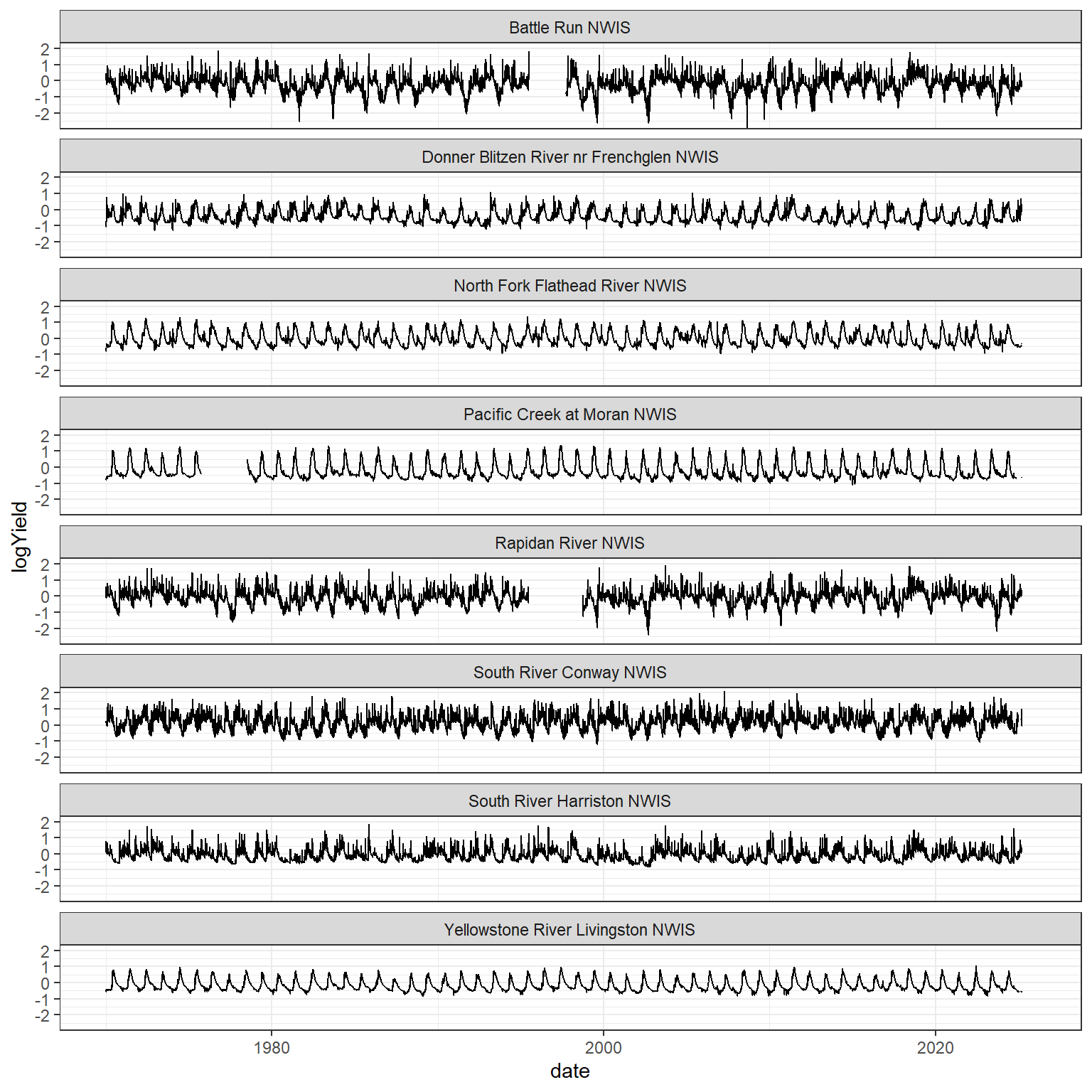
Download Daymet precip data and summarize by water year
# big G site lat/long
mysites <- nwis_daily %>% group_by(site_name, basin, subbasin, region) %>% summarize(lat = unique(lat), long = unique(long)) %>% ungroup()
# download point location Daymet data
climlist <- vector("list", length = dim(mysites)[1])
for (i in 1:dim(mysites)[1]) {
clim <- download_daymet(site = mysites$site_name[i], lat = mysites$lat[i], lon = mysites$long[i], start = 1980, end = 2024, internal = T)
climlist[[i]] <- tibble(clim$data) %>%
mutate(air_temp_mean = (tmax..deg.c. + tmin..deg.c.)/2,
date = as.Date(paste(year, yday, sep = "-"), "%Y-%j"),
site_name = mysites$site_name[i]) %>%
select(12,2,11,10,4,6) %>% rename(precip_mmday = 5, swe_kgm2 = 6)
print(i)
}[1] 1[1] 2[1] 3[1] 4[1] 5[1] 6[1] 7[1] 8# combine and add water years
climdf <- do.call(rbind, climlist) %>% left_join(mysites) %>% mutate(year = year(date))
climdf <- add_date_variables(climdf, dates = date, water_year_start = 10)
# calculate total annual precipitation in mm, by site and water year
climdf_summ <- climdf %>%
group_by(site_name, basin, subbasin, region, WaterYear) %>%
summarize(precip_total = sum(precip_mmday), sampsize = n()) %>%
mutate(precip_total_z = scale(precip_total)[,1]) %>%
ungroup() %>%
filter(sampsize >= 350)Write to file(s)
write_csv(climdf, "C:/Users/jbaldock/OneDrive - DOI/Documents/USGS/EcoDrought/EcoDrought Working/EcoDrought-Analysis/Qualitative/Daymet_climate.csv")
write_csv(climdf_summ, "C:/Users/jbaldock/OneDrive - DOI/Documents/USGS/EcoDrought/EcoDrought Working/EcoDrought-Analysis/Qualitative/Daymet_climate_summary.csv")Calculate annual water availability at big g as sum of daily yield values…retain only years with >95% data coverage (at least 350 days)
wateravail_sum <- dat_clean_big %>%
filter(!is.na(Yield_mm), Month %in% c(7:9)) %>%
group_by(basin, site_name, WaterYear) %>%
summarize(sampsize = n(), totalyield_sum = sum(Yield_mm, na.rm = TRUE)) %>%
mutate(totalyield_sum_z = scale(totalyield_sum)[,1]) %>%
ungroup() %>%
filter(sampsize >= 85) %>%
complete(basin, WaterYear = 1971:2024, fill = list(sampsize = NA, totalyield = NA)) %>%
select(-sampsize)
wateravail <- dat_clean_big %>%
filter(!is.na(Yield_mm)) %>%
group_by(basin, site_name, WaterYear) %>%
summarize(sampsize = n(), totalyield = sum(Yield_mm, na.rm = TRUE)) %>%
mutate(totalyield_z = scale(totalyield)[,1]) %>%
ungroup() %>%
filter(sampsize >= 350) %>%
complete(basin, WaterYear = 1971:2024, fill = list(sampsize = NA, totalyield = NA)) %>%
left_join(wateravail_sum)
# get range of years for little g data
daterange <- dat_clean %>% group_by(basin) %>% summarize(minyear = year(min(date)), maxyear = year(max(date)))
# spread ecod years
mylist <- vector("list", length = dim(daterange)[1])
for (i in 1:dim(daterange)[1]) {
mylist[[i]] <- tibble(basin = daterange$basin[i], WaterYear = seq(from = daterange$minyear[i], to = daterange$maxyear[i], by = 1))
}
yrdf <- do.call(rbind, mylist) %>% mutate(ecodyr = "yes")Write water availability to file
write_csv(wateravail, "C:/Users/jbaldock/OneDrive - DOI/Documents/USGS/EcoDrought/EcoDrought Working/EcoDrought-Analysis/Qualitative/BigG_wateravailability_annual.csv")View time series and scatter plots of big G water availability (total annual yield, sum of daily values, black lines) and precipitation (total annual precip, blues lines). Note that the panel labels indicate basins, not NWIS gage names. In the manuscript, pair these plots with CONUS map and detailed inset maps of focal basins (Figure 1)
ggplot() +
geom_rect(data = daterange, aes(xmin = minyear-0.5, xmax = maxyear+0.5, ymin = -Inf, ymax = +Inf), fill = "grey") +
geom_line(data = wateravail, aes(x = WaterYear, y = totalyield), linewidth = 1) +
geom_line(data = climdf_summ, aes(x = WaterYear, y = precip_total), linewidth = 0.5, col = "blue") +
facet_wrap(~basin) +
xlab("Water year") + ylab("Total annual yield (mm) / Total annual precipitation (mm)") +
theme_bw() + theme(panel.grid.major = element_blank(), panel.grid.minor = element_blank())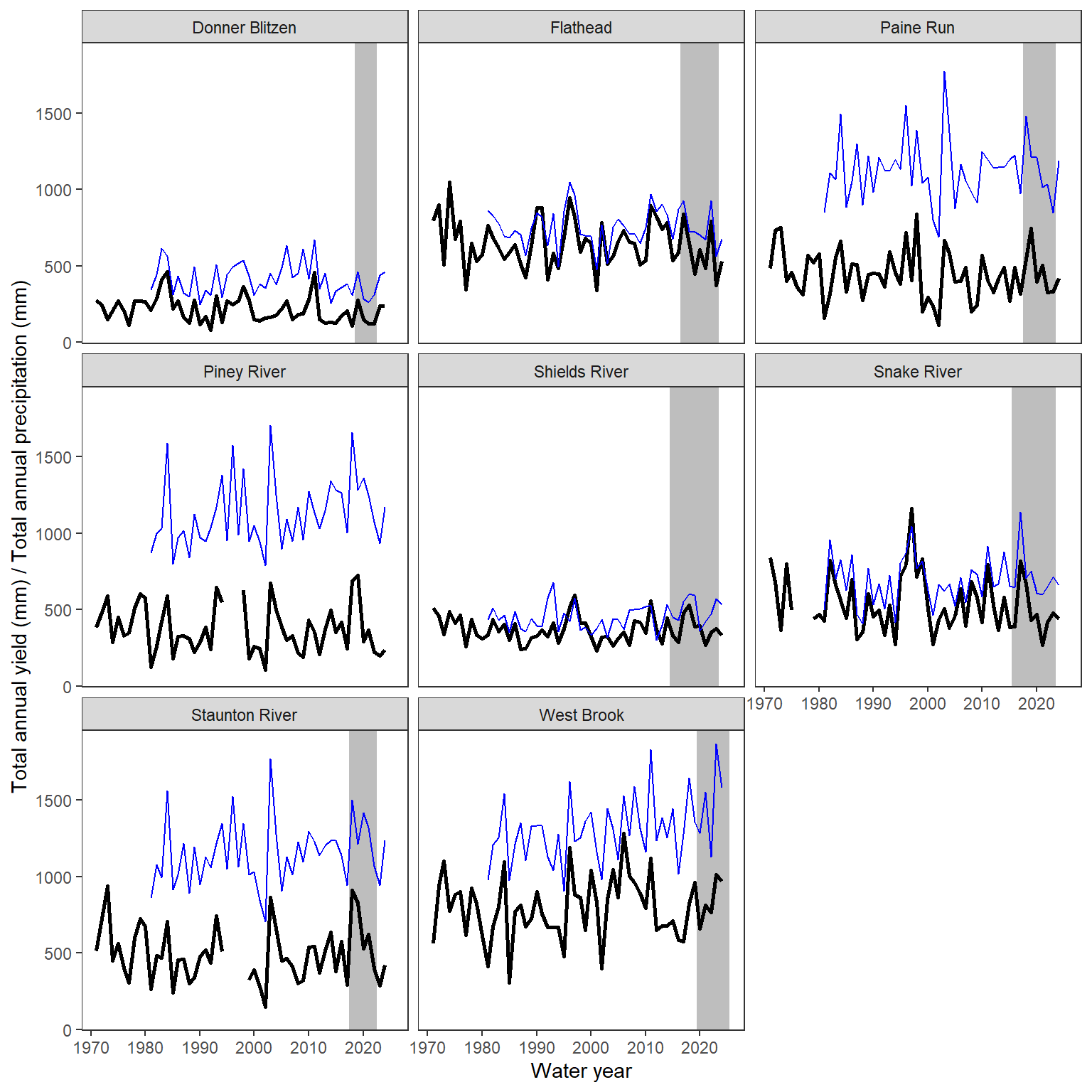
ggplot() +
geom_rect(data = daterange, aes(xmin = minyear-0.5, xmax = maxyear+0.5, ymin = -Inf, ymax = +Inf), fill = "grey") +
geom_line(data = wateravail, aes(x = WaterYear, y = totalyield_z), linewidth = 1) +
geom_line(data = climdf_summ, aes(x = WaterYear, y = precip_total_z), linewidth = 0.5, col = "blue") +
facet_wrap(~basin) +
xlab("Water year") + ylab("Total annual yield (scaled) / Total annual precipitation (scaled)") +
theme_bw() + theme(panel.grid.major = element_blank(), panel.grid.minor = element_blank())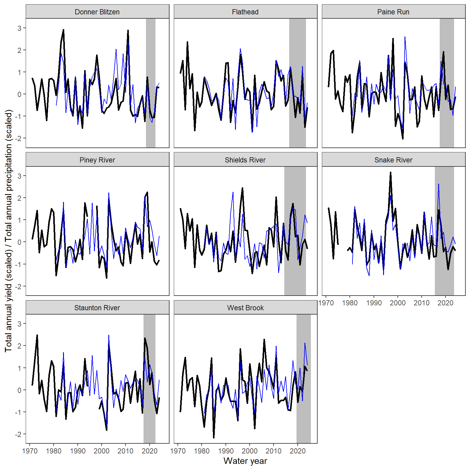
wateravail %>% select(-sampsize) %>% left_join(climdf_summ %>% select(-sampsize)) %>% left_join(yrdf) %>%
ggplot(aes(x = precip_total_z, y = totalyield_z)) +
geom_point(aes(color = ecodyr)) +
facet_wrap(~basin) +
xlab("Total annual precipitation (scaled)") + ylab("Total annual yield (scaled)") +
theme_bw() + theme(panel.grid.major = element_blank(), panel.grid.minor = element_blank(), legend.position = "none") +
stat_cor(method = "pearson", aes(label = ..r.label..))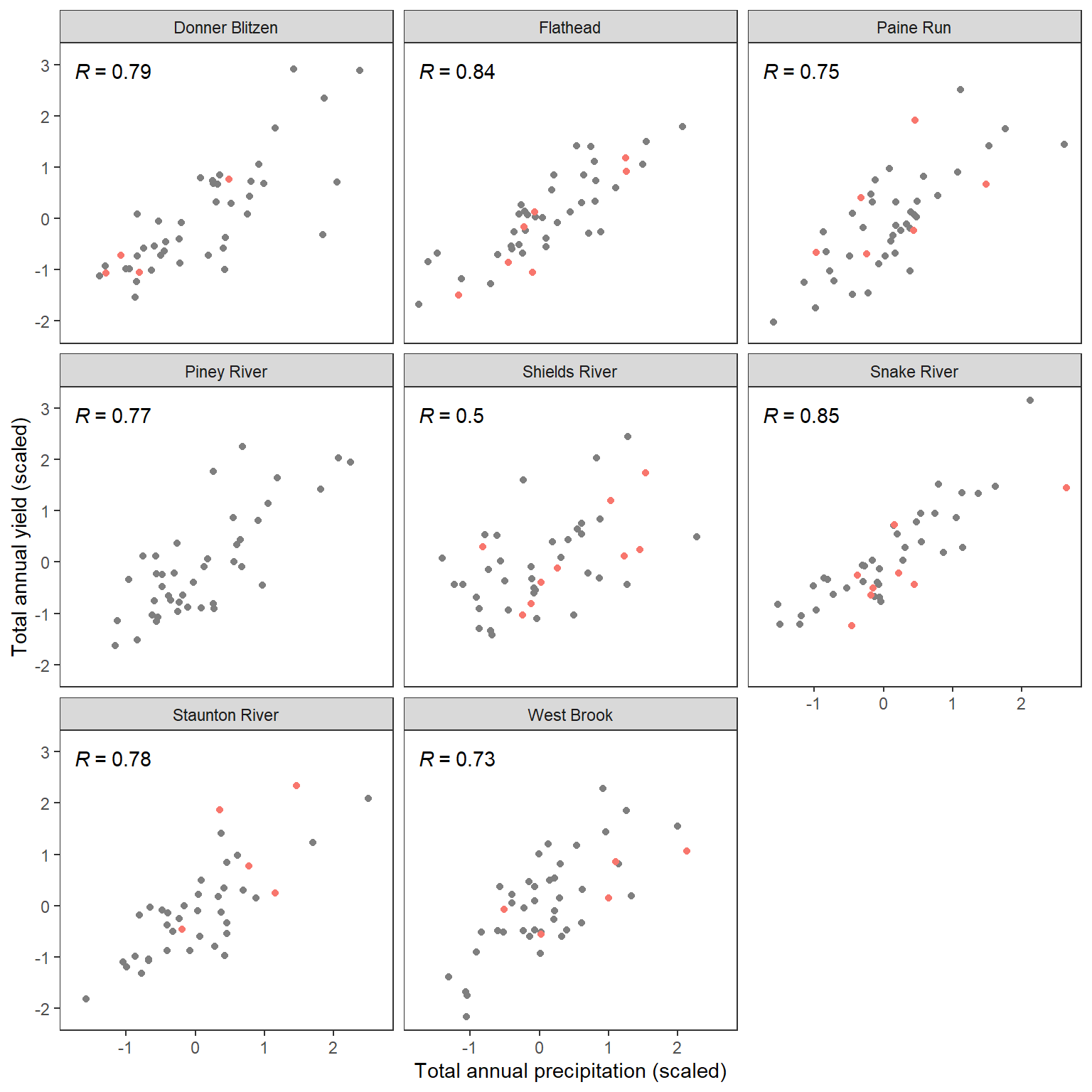
Load the NETCDF climate data and convert to usable/raster format
# Climate classification data loading and plotting in R
# Equivalent to the MATLAB script
library(ncdf4) # for reading NetCDF
library(terra) # for raster handling
library(ggplot2) # for plotting
library(rasterVis) # for nice levelplots of rasters
# library(rgdal) # for geotiff/geoshow equivalents
library(rgl)
# 1. Data import from NetCDF file
filename <- "C:/Users/jbaldock/OneDrive - DOI/Documents/USGS/EcoDrought/EcoDrought Working/Data/Spatial data/HydrologicClimateClassification.nc"
# Open NetCDF
nc <- nc_open(filename)
print(nc) # equivalent to MATLAB ncdispFile C:/Users/jbaldock/OneDrive - DOI/Documents/USGS/EcoDrought/EcoDrought Working/Data/Spatial data/HydrologicClimateClassification.nc (NC_FORMAT_NETCDF4_CLASSIC):
11 variables (excluding dimension variables):
double grid_aridity_Im[lat,lon] (Chunking: [360,720])
double grid_seasonalityOfAridity_Imr[lat,lon] (Chunking: [360,720])
double grid_annualSnowFraction_fs[lat,lon] (Chunking: [360,720])
double grid_latitude[lat,lon] (Chunking: [360,720])
double grid_longitude[lat,lon] (Chunking: [360,720])
double array_aridity_Im[length,width] (Chunking: [67214,1])
double array_seasonalityOfAridity_Imr[length,width] (Chunking: [67214,1])
double array_annualSnowFraction_fs[length,width] (Chunking: [67214,1])
double array_latitude[length,width] (Chunking: [67214,1])
double array_longitude[length,width] (Chunking: [67214,1])
double array_rgbColour[length,rgb] (Chunking: [67214,3])
5 dimensions:
lat Size:360 (no dimvar)
lon Size:720 (no dimvar)
length Size:67214 (no dimvar)
width Size:1 (no dimvar)
rgb Size:3 (no dimvar)# Variable names (must match those in the file)
varNames <- c(
"grid_aridity_Im",
"grid_seasonalityOfAridity_Imr",
"grid_annualSnowFraction_fs",
"grid_latitude",
"grid_longitude",
"array_aridity_Im",
"array_seasonalityOfAridity_Imr",
"array_annualSnowFraction_fs",
"array_latitude",
"array_longitude",
"array_rgbColour"
)
# Extract variables into a list (like a struct in MATLAB)
ClimateClassification <- lapply(varNames, function(v) ncvar_get(nc, v))
names(ClimateClassification) <- varNames
nc_close(nc)
# 2a. Example maps of gridded climate indices ----------------------------
# Wrap into SpatRaster objects (terra) for plotting
grid_Im <- rast(ClimateClassification$grid_aridity_Im)
grid_Imr <- rast(ClimateClassification$grid_seasonalityOfAridity_Imr)
grid_fs <- rast(ClimateClassification$grid_annualSnowFraction_fs)
# Assign CRS and extent (need to use lat/lon arrays)
lat <- ClimateClassification$grid_latitude
lon <- ClimateClassification$grid_longitude
ext(grid_Im) <- c(min(lon), max(lon), min(lat), max(lat))
crs(grid_Im) <- "EPSG:4326"
ext(grid_Imr) <- ext(grid_Im); crs(grid_Imr) <- "EPSG:4326"
ext(grid_fs) <- ext(grid_Im); crs(grid_fs) <- "EPSG:4326"
# correct orientation
grid_Im <- flip(grid_Im, direction = "vertical")
grid_Imr <- flip(grid_Imr, direction = "vertical")
grid_fs <- flip(grid_fs, direction = "vertical")
# Plot rasters
levelplot(grid_Im, margin = FALSE, main = "Aridity index I_m",
at = seq(-1, 1, 0.1), col.regions = viridis::viridis(20))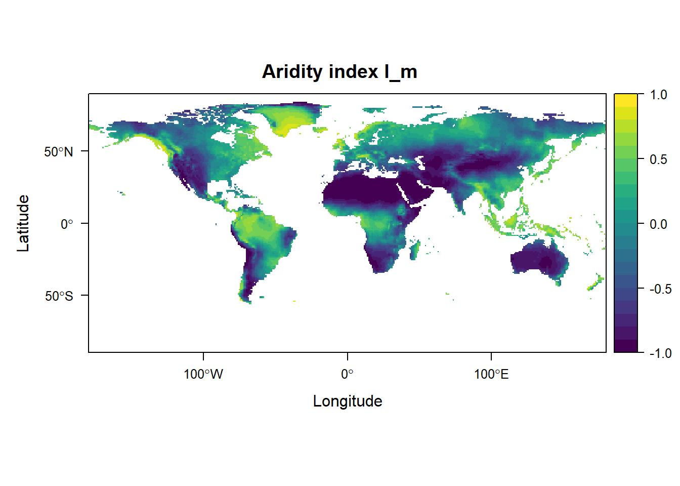
levelplot(grid_Imr, margin = FALSE, main = "Aridity seasonality index I_{m,r}",
at = seq(0, 2, 0.1), col.regions = viridis::viridis(20))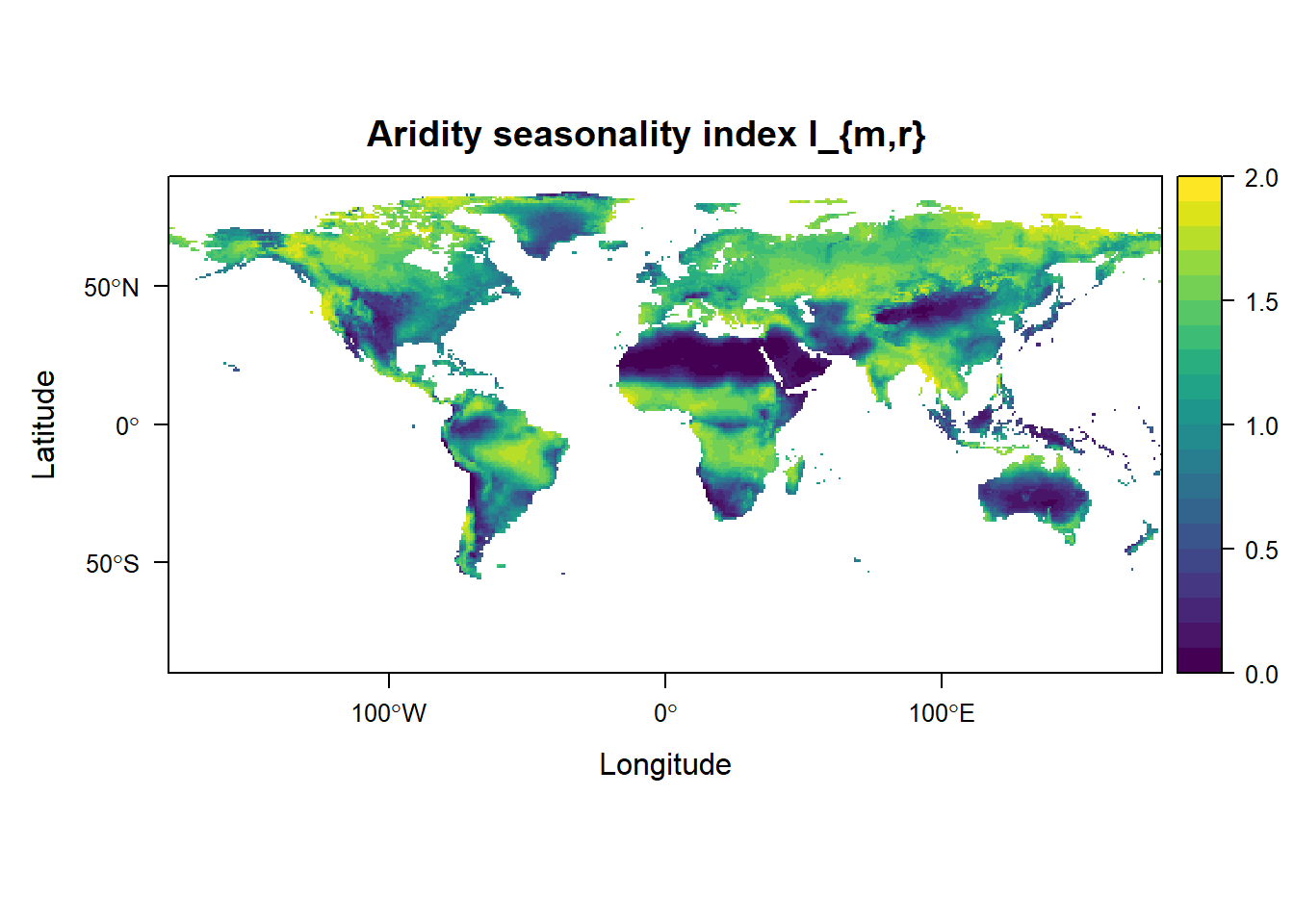
levelplot(grid_fs, margin = FALSE, main = "Fraction precipitation as snow f_s",
at = seq(0, 1, 0.05), col.regions = viridis::viridis(20))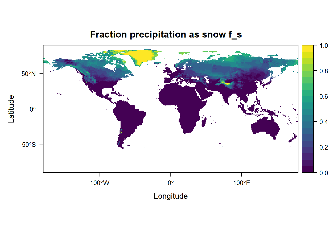
# 2b. Combined climate map -----------------------------------------------
df_array <- data.frame(
lon = ClimateClassification$array_longitude,
lat = ClimateClassification$array_latitude,
col = rgb(
ClimateClassification$array_rgbColour[,1],
ClimateClassification$array_rgbColour[,2],
ClimateClassification$array_rgbColour[,3],
maxColorValue = 1
)
)
ggplot(df_array, aes(x = lon, y = lat, color = col)) +
geom_point(size = 0.5) +
scale_color_identity() +
coord_equal() +
theme_minimal() +
labs(title = "Climatic gradients from climate indices")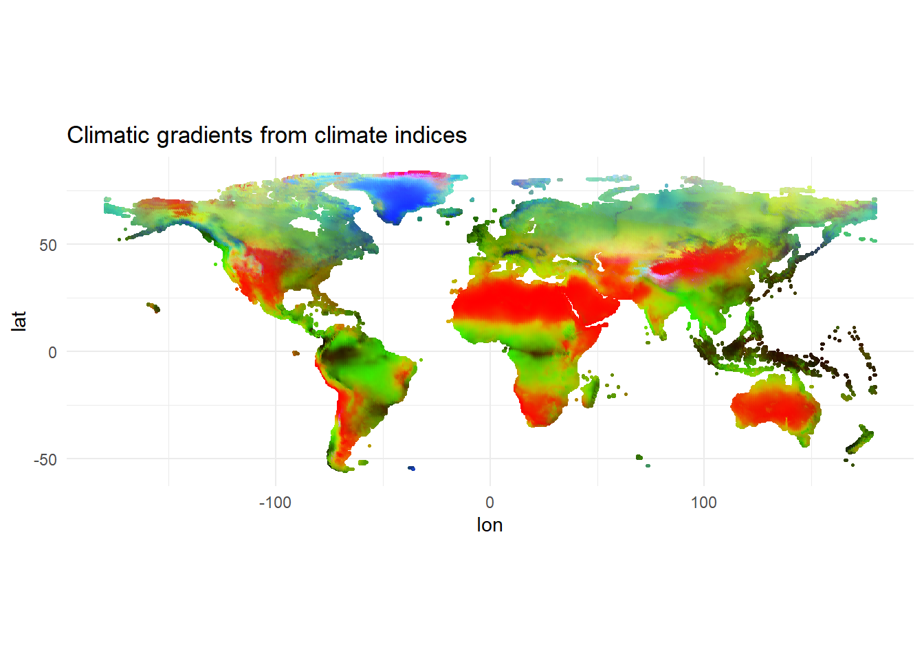
# 2c. RGB colour legend (3D scatterplot) ---------------------------------
df_legend <- data.frame(
Im = ClimateClassification$array_aridity_Im,
Imr = ClimateClassification$array_seasonalityOfAridity_Imr,
fs = ClimateClassification$array_annualSnowFraction_fs,
col = df_array$col
)
# Using plotly for interactive 3D equivalent of MATLAB scatter3
library(plotly)
library(orca)
plot_ly(df_legend, x = ~Im, y = ~Imr, z = ~fs,
type = "scatter3d", mode = "markers",
marker = list(color = df_legend$col, size = 2, opacity = 0.5)) %>%
layout(scene = list(
xaxis = list(title = "Aridity"),
yaxis = list(title = "Seasonality"),
zaxis = list(title = "Snow fraction")
))plot_ly(df_legend, x = ~Im, y = ~Imr, z = ~fs,
type = "scatter3d", mode = "markers",
marker = list(color = "grey", size = 2, opacity = 0.5)) %>%
layout(scene = list(
xaxis = list(title = "Aridity"),
yaxis = list(title = "Seasonality"),
zaxis = list(title = "Snow fraction")
))# 2d. GeoTIFF plot of the main map ---------------------------------------
# geofile <- "C:/Users/jbaldock/OneDrive - DOI/Documents/USGS/EcoDrought/EcoDrought Working/Data/Spatial data/ClimateClassification_mainMap_geoReferenced.tif"
# map_rast <- rast(geofile)
#
# plot(map_rast, main = "Climatic gradients from climate indices")Stack rasters and extract values for focal sites
# combine the climate variables into a raster stack
# add 1 to Im to force positive (needed for expansion factors)
climate_stack <- c(grid_Im+1, grid_Imr, grid_fs)
names(climate_stack) <- c("Im", "Imr", "fs")
# convert to tibble
climate_df <- tidyterra::as_tibble(climate_stack)
# hydroclidf_noNA <- as_tibble(hydrocli) %>% filter(!is.na(aridity))
summary(climate_df) Im Imr fs
Min. :0.000 Min. :0.000 Min. :0.000
1st Qu.:0.360 1st Qu.:0.736 1st Qu.:0.000
Median :0.809 Median :1.270 Median :0.044
Mean :0.805 Mean :1.110 Mean :0.200
3rd Qu.:1.222 3rd Qu.:1.526 3rd Qu.:0.361
Max. :1.880 Max. :2.000 Max. :1.000
NA's :191986 NA's :191986 NA's :191986 # get site location data
sitevec <- vect(focalsites)
# extract climate data for each site
extracted_vals <- extract(climate_stack, sitevec)
range(extracted_vals$Im)[1] 0.217410 1.304555range(extracted_vals$Imr)[1] 0.6266317 1.5323583range(extracted_vals$fs)[1] 0.0000000 0.4364088Get centroid from base hull
hull <- convhulln(extracted_vals[,-1])
hull_vertices <- extracted_vals[unique(as.vector(hull)), ]
centroid <- colMeans(hull_vertices[,-1])Test pit: develop code to expand and estimate convex hulls, subset global points, and plot in 3d
# set expansion factor
scf <- 2
# define hull
pts_expanded <- sweep(sweep(extracted_vals[,-1], 2, centroid, "-") * scf, 2, centroid, "+")
hull_indices <- geometry::convhulln(pts_expanded)
# subset global points in hull
points_in_hull <- inhulln(hull_indices, as.matrix(climate_df))
points_in_hull_num <- as.numeric(points_in_hull)
# points_in_hull_num[points_in_hull_num == 0] <- NA
# create new hydroclimate envelope layer
new_layer <- rast(climate_stack[[1]], vals = points_in_hull_num)
names(new_layer) <- "myhc"
# plot(new_layer)
#
# hydroclidf <- as_tibble(c(climate_stack, new_layer)) %>%
# filter(!is.na(myhc)) %>%
# # mutate(myhc = as.numeric(points_in_hull)) %>%
# # mutate(myhc = if_else(is.na(snowfrac), NA, myhc)) %>%
# mutate(color = if_else(myhc == 1, "red", if_else(myhc == 0, "grey", NA)))
hydroclidf <- as_tibble(c(climate_stack, new_layer)) %>%
filter(myhc == 1)
# rgl::plot3d(x = hydroclidf$Im, y = hydroclidf$Imr, z = hydroclidf$fs, col = hydroclidf$color)
plot_ly() %>%
add_markers(
data = climate_df,
x = ~Im, y = ~Imr, z = ~fs,
marker = list(size = 1, opacity = 0.2, color = "grey"),
name = "All points"
) %>%
# Add highlighted global points in hull
add_markers(
data = hydroclidf,
x = ~Im, y = ~Imr, z = ~fs,
marker = list(size = 1, opacity = 0.5, color = "blue"),
name = "All points"
) %>%
#Add highlighted subset of points with different style
add_markers(
data = extracted_vals,
x = ~Im, y = ~Imr, z = ~fs,
marker = list(size = 5, opacity = 0.8, color = "black", symbol = "circle"),
name = "Highlighted points"
) %>%
layout(
scene = list(
xaxis = list(title = "Aridity"),
yaxis = list(title = "Seasonality"),
zaxis = list(title = "Snow fraction")
)
)Subset global climate data using 3d convex hull fit to focal sites, with different percentage expansion factors.
scale_factor <- seq(from = 1, to = 2, by = 0.1)
new_layer_list_raw <- list()
new_layer_list <- list()
for (i in 1:length(scale_factor)) {
# Expand all original points relative to centroid
pts_expanded <- sweep(sweep(extracted_vals[,-1], 2, centroid, "-") * scale_factor[i], 2, centroid, "+")
# recompute convex hull
hull_expanded <- geometry::convhulln(pts_expanded)
# subset points/raster cells
points_in_hull <- geometry::inhulln(hull_expanded, as.matrix(climate_df))
points_in_hull_num <- as.numeric(points_in_hull)
# create layer and save in list (for 3-d scatterplots and hulls)
new_layer <- rast(climate_stack[[1]], vals = points_in_hull_num)
names(new_layer) <- paste("expand_", scale_factor[i], sep = "")
new_layer_list_raw[[i]] <- new_layer
# for mapping, we need to set the 0's (cells not in hydroclimate zone) to NA
points_in_hull_num[points_in_hull_num == 0] <- NA
# create layer and save in list (for mapping)
new_layer <- rast(climate_stack[[1]], vals = points_in_hull_num)
names(new_layer) <- paste("expand_", scale_factor[i], sep = "")
new_layer_list[[i]] <- new_layer
}Draw the map
mypal <- hcl.colors(length(scale_factor), palette = "Emrld")
maps::map("world", col="grey", fill=TRUE, lwd = 0.2, mar = c(0,0,0,5))
# box()
for (i in rev(1:length(scale_factor))) {
plot(new_layer_list[[i]], add = TRUE, col = mypal[i], legend = FALSE)
}
maps::map("world", col = NA, fill=TRUE, add = TRUE, lwd = 0.2, mar = c(0,0,0,5))
legend("right", legend = scale_factor, fill = mypal, title = "Hydroclimatic\nenvelope\n(exp. factor)", bty = "n", xpd = TRUE, inset = c(-0.05,0), cex = 0.8)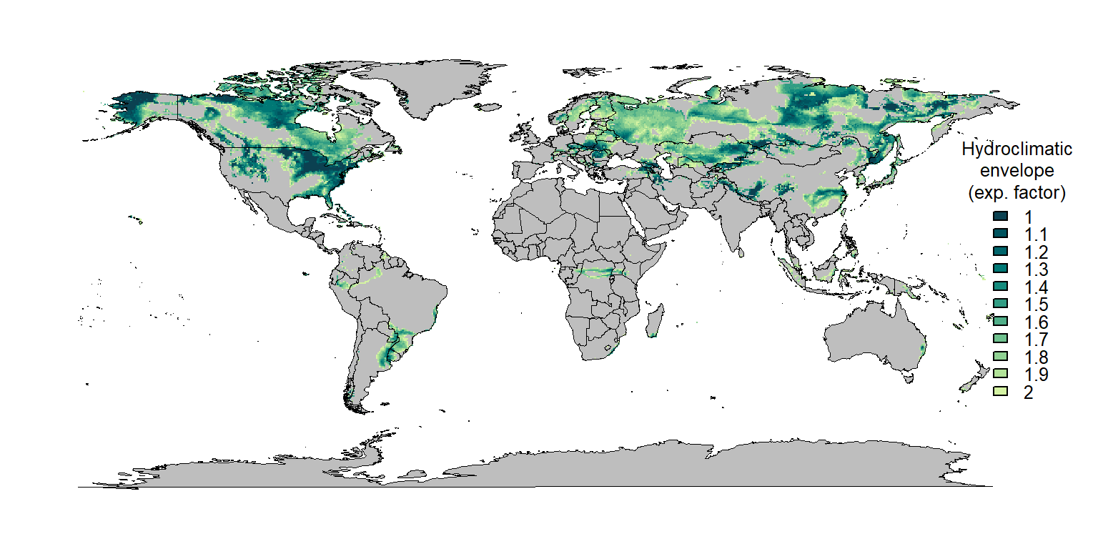
Write to file
# color palette
mypal <- hcl.colors(length(scale_factor), palette = "Emrld")
# write plot to file
jpeg("C:/Users/jbaldock/OneDrive - DOI/Documents/USGS/EcoDrought/EcoDrought Working/Presentation figs/Fig1_WorldMap_ClimateContext_REDO.jpg", width = 8, height = 4, units = "in", res = 1000)
# par(mar = c(0,0,0,10), xpd = TRUE)
maps::map("world", col="grey", fill=TRUE, lwd = 0.2, mar = c(0,0,0,5))
# box()
for (i in rev(1:length(scale_factor))) {
plot(new_layer_list[[i]], add = TRUE, col = mypal[i], legend = FALSE)
}
maps::map("world", col = NA, fill=TRUE, add = TRUE, lwd = 0.2, mar = c(0,0,0,5))
legend("right", legend = scale_factor, fill = mypal, title = "Hydroclimatic\nenvelope\n(exp. factor)", bty = "n", xpd = TRUE, inset = c(-0.05,0), cex = 0.8)
dev.off()png
2 Draw 3-d scatterplots with envelopes
mylayer <- new_layer_list_raw[[1]]
names(mylayer) <- "myhc"
hydroclidf <- as_tibble(c(climate_stack, mylayer)) %>%
filter(!is.na(fs)) %>%
# mutate(myhc = as.numeric(points_in_hull)) %>%
# mutate(myhc = if_else(is.na(snowfrac), NA, myhc)) %>%
mutate(color = if_else(myhc == 1, "red", if_else(myhc == 0, "grey", NA)))
scatterplot3d(hydroclidf[,c(1:3)], color = hydroclidf$color, pch = 16, cex.symbols = 0.2, grid = FALSE, angle = 50)
rgl::plot3d(x = hydroclidf$Im, y = hydroclidf$Imr, z = hydroclidf$fs, col = hydroclidf$color)# define color palette
mycols <- brewer.pal(7, "Set2")
coltib <- tibble(basin = c("West Brook", "Staunton River", "Paine Run", "Flathead River", "Yellowstone River", "Snake River", "Donner und Blitzen River"),
color = brewer.pal(7, "Set2"))
# reconfigure extracted values (focal sites)
extracted_vals2 <- tibble(extracted_vals) %>%
mutate(basin = recode(focalsites$basin, "Shields River" = "Yellowstone River", "Flathead" = "Flathead River", "Donner Blitzen" = "Donner und Blitzen River")) %>%
left_join(coltib) %>%
mutate(Im = Im - 1)
# color points in hull, expansion factor = 1.0
mylayer <- new_layer_list_raw[[1]]
names(mylayer) <- "myhc"
hydroclidf_1 <- as_tibble(c(climate_stack, mylayer)) %>%
filter(myhc == 1) %>% mutate(Im = Im-1)
# color points in hull, expansion factor = 1.5
mylayer <- new_layer_list_raw[[11]]
names(mylayer) <- "myhc"
hydroclidf_2 <- as_tibble(c(climate_stack, mylayer)) %>%
filter(myhc == 1) %>% mutate(Im = Im-1)
# Start with the base scatter of all points
p <- plot_ly() %>%
add_markers(
data = df_legend,
x = ~Im, y = ~Imr, z = ~fs,
marker = list(size = 1, opacity = 0.2, color = "grey"),
name = "All points"
) %>%
#Add convex hull mesh
# add_trace(
# type = "mesh3d",
# x = pts[hull,1], y = pts[hull,2], z = pts[hull,3],
# i = hull[,1]-1, j = hull[,2]-1, k = hull[,3]-1, # zero-based indexing
# opacity = 0.2,
# color = I("red"),
# name = "Convex hull"
# ) %>%
# Add highlighted global points in hull
add_markers(
data = hydroclidf_1,
x = ~Im, y = ~Imr, z = ~fs,
marker = list(size = 1, opacity = 0.3, color = "black"),
name = "All points"
) %>%
#Add highlighted subset of points with different style
add_markers(
data = extracted_vals2,
x = ~Im, y = ~Imr, z = ~fs,
marker = list(size = 5, opacity = 0.8, color = extracted_vals2$color, symbol = "circle"),
name = "Highlighted points"
) %>%
layout(
scene = list(
xaxis = list(title = "Aridity"),
yaxis = list(title = "Seasonality"),
zaxis = list(title = "Snow fraction")
)
)
pStatic 3d scatterplot
par(mar = c(2,2,2,2), mgp = c(5,1,0))
scatter3D(x = df_legend$Im, y = df_legend$Imr, z = df_legend$fs,
col = alpha("grey", 0.2), cex = 0.15, pch = 16, bty = "b2",
xlab = "", ylab = "", zlab = "",
phi = 25, theta = -50, expand = 0.75, ticktype = "detailed")
scatter3D(x = extracted_vals2$Im, y = extracted_vals2$Imr, z = extracted_vals2$fs-0.03,
col = "black", type = "h", add = TRUE, pch = NA)
scatter3D(x = extracted_vals2$Im, y = extracted_vals2$Imr, z = extracted_vals2$fs,
bg = extracted_vals2$color, col = "black", cex = 1.5, pch = 21, add = TRUE)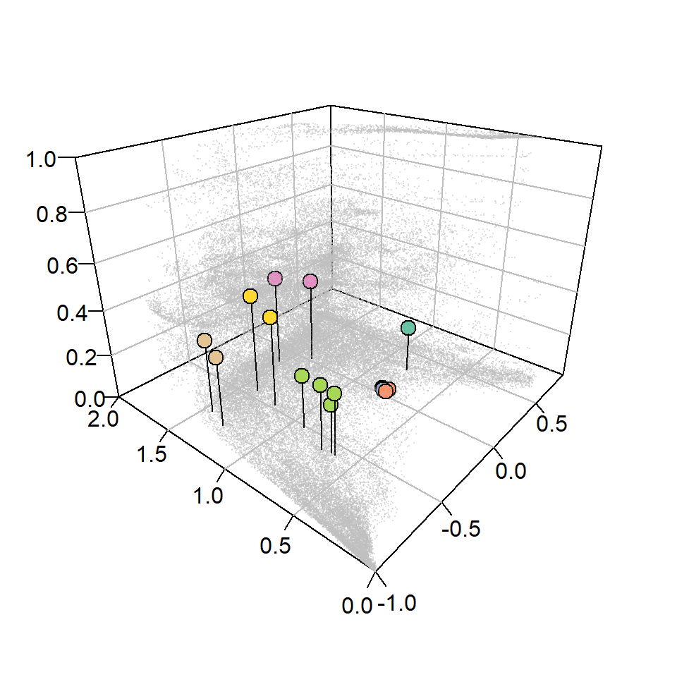
Write 3d scatterplots to file
jpeg("C:/Users/jbaldock/OneDrive - DOI/Documents/USGS/EcoDrought/EcoDrought Working/Presentation figs/Fig1_3Dscatter_NoHull.jpg", width = 5, height = 5, units = "in", res = 1000)
par(mar = c(2,2,2,2), mgp = c(5,1,0))
scatter3D(x = df_legend$Im, y = df_legend$Imr, z = df_legend$fs,
col = alpha("grey", 0.2), cex = 0.15, pch = 16, bty = "b2",
xlab = "", ylab = "", zlab = "",
phi = 25, theta = -50, expand = 0.75, ticktype = "detailed")
scatter3D(x = extracted_vals2$Im, y = extracted_vals2$Imr, z = extracted_vals2$fs-0.03,
col = "black", type = "h", add = TRUE, pch = NA)
scatter3D(x = extracted_vals2$Im, y = extracted_vals2$Imr, z = extracted_vals2$fs,
bg = extracted_vals2$color, col = "black", cex = 1.5, pch = 21, add = TRUE)
dev.off()
jpeg("C:/Users/jbaldock/OneDrive - DOI/Documents/USGS/EcoDrought/EcoDrought Working/Presentation figs/Fig1_3Dscatter_basehull.jpg", width = 5, height = 5, units = "in", res = 1000)
par(mar = c(2,2,2,2), mgp = c(5,1,0))
scatter3D(x = df_legend$Im, y = df_legend$Imr, z = df_legend$fs,
col = alpha("grey", 0.2), cex = 0.15, pch = 16, bty = "b2",
xlab = "", ylab = "", zlab = "",
phi = 25, theta = -50, expand = 0.75, ticktype = "detailed")
scatter3D(x = hydroclidf_1$Im, y = hydroclidf_1$Imr, z = hydroclidf_1$fs,
col = alpha("black", 0.4), cex = 0.2, pch = 16, add = TRUE)
scatter3D(x = extracted_vals2$Im, y = extracted_vals2$Imr, z = extracted_vals2$fs,
bg = extracted_vals2$color, col = "black", cex = 1.5, pch = 21, add = TRUE)
dev.off()
jpeg("C:/Users/jbaldock/OneDrive - DOI/Documents/USGS/EcoDrought/EcoDrought Working/Presentation figs/Fig1_3Dscatter_BIGhull.jpg", width = 5, height = 5, units = "in", res = 1000)
par(mar = c(2,2,2,2), mgp = c(5,1,0))
scatter3D(x = df_legend$Im, y = df_legend$Imr, z = df_legend$fs,
col = alpha("grey", 0.2), cex = 0.15, pch = 16, bty = "b2",
xlab = "", ylab = "", zlab = "",
phi = 25, theta = -50, expand = 0.75, ticktype = "detailed")
scatter3D(x = hydroclidf_2$Im, y = hydroclidf_2$Imr, z = hydroclidf_2$fs,
col = alpha("black", 0.4), cex = 0.2, pch = 16, add = TRUE)
scatter3D(x = extracted_vals2$Im, y = extracted_vals2$Imr, z = extracted_vals2$fs,
bg = extracted_vals2$color, col = "black", cex = 1.5, pch = 21, add = TRUE)
dev.off()View global and focal site distributions of climate data
par(mfrow = c(3,1), mar = c(2.5,0.5,0.1,0.5), mgp = c(1.5,0.5,0), xpd = TRUE)
dens <- density(df_legend$Im)
plot(dens, type = "n", xlab = "Aridity", ylab = "", main = "", bty = "n", xlim = c(-1, 1), axes = FALSE)
polygon(dens, col = "grey70", border = NA)
lines(dens, bty = "n")
polygon(x = c(-10, -1, -1, -10), y = c(-10, -10, 10, 10), border = NA, col = "white")
polygon(x = c(10, 1, 1, 10), y = c(-10, -10, 10, 10), border = NA, col = "white")
axis(1)
points(x = jitter(extracted_vals2$Im, factor = 20), y = rep(0, times = dim(extracted_vals2)[1]), pch = 21, bg = extracted_vals2$color, cex = 2)
dens <- density(df_legend$Imr)
plot(dens, type = "n", xlab = "Seasonality", ylab = "", main = "", bty = "n", xlim = c(0, 2), axes = FALSE)
polygon(dens, col = "grey70", border = NA)
lines(dens, bty = "n")
polygon(x = c(-10, 0, 0, -10), y = c(-10, -10, 10, 10), border = NA, col = "white")
polygon(x = c(10, 2, 2, 10), y = c(-10, -10, 10, 10), border = NA, col = "white")
axis(1)
points(x = jitter(extracted_vals2$Imr, factor = 20), y = rep(0, times = dim(extracted_vals2)[1]), pch = 21, bg = extracted_vals2$color, cex = 2)
dens <- density(df_legend$fs)
plot(dens, type = "n", xlab = "Precipitation as snow", ylab = "", main = "", bty = "n", xlim = c(0, 1), axes = FALSE)
polygon(dens, col = "grey70", border = NA)
lines(dens, bty = "n")
polygon(x = c(-10, 0, 0, -10), y = c(-10, -10, 10, 10), border = NA, col = "white")
polygon(x = c(10, 1, 1, 10), y = c(-10, -10, 10, 10), border = NA, col = "white")
axis(1)
points(x = jitter(extracted_vals2$fs, factor = 20), y = rep(0, times = dim(extracted_vals2)[1]), pch = 21, bg = extracted_vals2$color, cex = 2)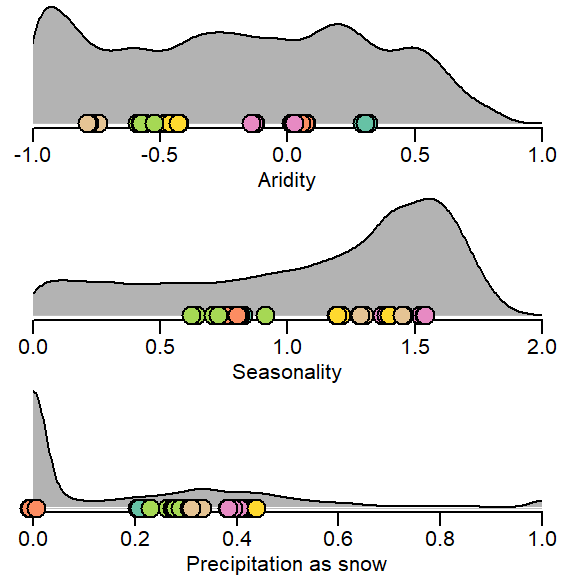
Write to file
jpeg("C:/Users/jbaldock/OneDrive - DOI/Documents/USGS/EcoDrought/EcoDrought Working/Presentation figs/Fig1_ClimateDensityDistributions2.jpg", width = 3, height = 3, units = "in", res = 1000)
par(mfrow = c(3,1), mar = c(2.5,0.5,0.1,0.5), mgp = c(1.5,0.5,0), xpd = TRUE)
dens <- density(df_legend$Im)
plot(dens, type = "n", xlab = "Aridity", ylab = "", main = "", bty = "n", xlim = c(-1, 1), axes = FALSE)
polygon(dens, col = "grey70", border = NA)
lines(dens, bty = "n")
polygon(x = c(-10, -1, -1, -10), y = c(-10, -10, 10, 10), border = NA, col = "white")
polygon(x = c(10, 1, 1, 10), y = c(-10, -10, 10, 10), border = NA, col = "white")
axis(1)
points(x = jitter(extracted_vals2$Im, factor = 20), y = rep(0, times = dim(extracted_vals2)[1]), pch = 21, bg = extracted_vals2$color, cex = 2)
dens <- density(df_legend$Imr)
plot(dens, type = "n", xlab = "Seasonality", ylab = "", main = "", bty = "n", xlim = c(0, 2), axes = FALSE)
polygon(dens, col = "grey70", border = NA)
lines(dens, bty = "n")
polygon(x = c(-10, 0, 0, -10), y = c(-10, -10, 10, 10), border = NA, col = "white")
polygon(x = c(10, 2, 2, 10), y = c(-10, -10, 10, 10), border = NA, col = "white")
axis(1)
points(x = jitter(extracted_vals2$Imr, factor = 20), y = rep(0, times = dim(extracted_vals2)[1]), pch = 21, bg = extracted_vals2$color, cex = 2)
dens <- density(df_legend$fs)
plot(dens, type = "n", xlab = "Precipitation as snow", ylab = "", main = "", bty = "n", xlim = c(0, 1), axes = FALSE)
polygon(dens, col = "grey70", border = NA)
lines(dens, bty = "n")
polygon(x = c(-10, 0, 0, -10), y = c(-10, -10, 10, 10), border = NA, col = "white")
polygon(x = c(10, 1, 1, 10), y = c(-10, -10, 10, 10), border = NA, col = "white")
axis(1)
points(x = jitter(extracted_vals2$fs, factor = 20), y = rep(0, times = dim(extracted_vals2)[1]), pch = 21, bg = extracted_vals2$color, cex = 2)
dev.off()Plot monthly estimates of repeatability by climate indices
mysites <- as_tibble(focalsites) %>%
mutate(Im = extracted_vals$Im,
Imr = extracted_vals$Imr,
fs = extracted_vals$fs) %>%
group_by(basin) %>%
summarize(Im = mean(Im), Imr = mean(Imr), fs = mean(fs)) %>%
ungroup() %>%
filter(basin != "Donner Blitzen") %>%
mutate(basin = ifelse(basin == "Paine Run", "Paine",
ifelse(basin == "Staunton River", "Staunton",
ifelse(basin == "Snake River", "Snake",
ifelse(basin == "Shields River", "Yellowstone", basin))))) %>%
mutate(basin = factor(basin, levels = rev(c("West Brook", "Staunton", "Paine", "Flathead", "Yellowstone", "Snake")))) %>%
mutate(R = c(0.55, 0.56, 0.71, 0.94, 0.44, 0.47))
ggpairs(mysites)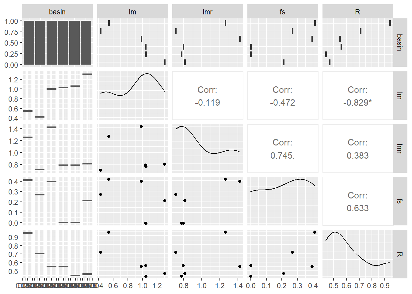
Plot
myr <- cor(mysites$Im, mysites$R)
mysites %>% ggplot(aes(x = Im, y = R)) +
geom_point(aes(fill = basin), shape = 21, size = 3) +
annotate("text", x = Inf, y = Inf, hjust = 1.1, vjust = 1.5,
label = paste("Pearson's r = ", round(myr, digits = 2))) +
scale_fill_manual(values = rev(brewer.pal(6, "Set2"))) +
theme_bw() + theme(legend.position = "none", panel.grid = element_blank(),
axis.text = element_text(color = "black")) +
xlab("Aridity") + ylab("Median repeatability (R)")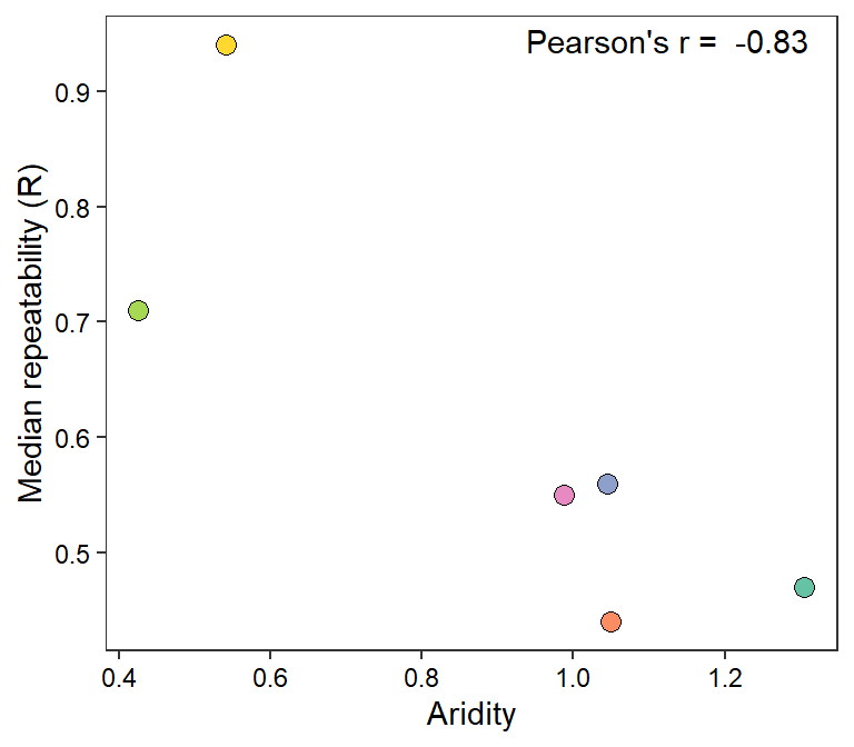
myr <- cor(mysites$Imr, mysites$R)
mysites %>% ggplot(aes(x = Imr, y = R)) +
geom_point(aes(fill = basin), shape = 21, size = 3) +
annotate("text", x = -Inf, y = Inf, hjust = -0.1, vjust = 1.5,
label = paste("Pearson's r = ", round(myr, digits = 2))) +
scale_fill_manual(values = rev(brewer.pal(6, "Set2"))) +
theme_bw() + theme(legend.position = "none", panel.grid = element_blank(),
axis.text = element_text(color = "black")) +
xlab("Seasonality") + ylab("Median repeatability (R)")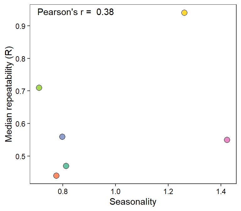
myr <- cor(mysites$fs, mysites$R)
mysites %>% ggplot(aes(x = fs, y = R)) +
geom_point(aes(fill = basin), shape = 21, size = 3) +
annotate("text", x = -Inf, y = Inf, hjust = -0.1, vjust = 1.5,
label = paste("Pearson's r = ", round(myr, digits = 2))) +
scale_fill_manual(values = rev(brewer.pal(6, "Set2"))) +
theme_bw() + theme(legend.position = "none", panel.grid = element_blank(),
axis.text = element_text(color = "black")) +
xlab("Precipitation as snow") + ylab("Median repeatability (R)")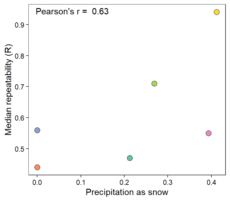
Write to file
jpeg("C:/Users/jbaldock/OneDrive - DOI/Documents/USGS/EcoDrought/EcoDrought Working/Presentation figs/Repeatability_Aridity.jpg", width = 4, height = 3.5, units = "in", res = 1000)
myr <- cor(mysites$Im, mysites$R)
mysites %>% ggplot(aes(x = Im, y = R)) +
geom_point(aes(fill = basin), shape = 21, size = 3) +
annotate("text", x = Inf, y = Inf, hjust = 1.1, vjust = 1.5,
label = paste("Pearson's r = ", round(myr, digits = 2))) +
scale_fill_manual(values = rev(brewer.pal(6, "Set2"))) +
theme_bw() + theme(legend.position = "none", panel.grid = element_blank(),
axis.text = element_text(color = "black")) +
xlab("Aridity") + ylab("Median repeatability (R)")
dev.off()png
2 jpeg("C:/Users/jbaldock/OneDrive - DOI/Documents/USGS/EcoDrought/EcoDrought Working/Presentation figs/Repeatability_Seasonality.jpg", width = 4, height = 3.5, units = "in", res = 1000)
myr <- cor(mysites$Imr, mysites$R)
mysites %>% ggplot(aes(x = Imr, y = R)) +
geom_point(aes(fill = basin), shape = 21, size = 3) +
annotate("text", x = -Inf, y = Inf, hjust = -0.1, vjust = 1.5,
label = paste("Pearson's r = ", round(myr, digits = 2))) +
scale_fill_manual(values = rev(brewer.pal(6, "Set2"))) +
theme_bw() + theme(legend.position = "none", panel.grid = element_blank(),
axis.text = element_text(color = "black")) +
xlab("Seasonality") + ylab("Median repeatability (R)")
dev.off()png
2 jpeg("C:/Users/jbaldock/OneDrive - DOI/Documents/USGS/EcoDrought/EcoDrought Working/Presentation figs/Repeatability_SnowFraction.jpg", width = 4, height = 3.5, units = "in", res = 1000)
myr <- cor(mysites$fs, mysites$R)
mysites %>% ggplot(aes(x = fs, y = R)) +
geom_point(aes(fill = basin), shape = 21, size = 3) +
annotate("text", x = -Inf, y = Inf, hjust = -0.1, vjust = 1.5,
label = paste("Pearson's r = ", round(myr, digits = 2))) +
scale_fill_manual(values = rev(brewer.pal(6, "Set2"))) +
theme_bw() + theme(legend.position = "none", panel.grid = element_blank(),
axis.text = element_text(color = "black")) +
xlab("Precipitation as snow") + ylab("Median repeatability (R)")
dev.off()png
2