11 Hysteresis

Purpose: Explore non-linear and hysteretic relationship between flow at reference vs. at headwater gages

Approach:

Trim data to complete site-years.
Use scatterplots to show diversity in g~G relationships within and among basins.
Conduct event delineation and calculate the (modified) Lloyd index for each g~G pair of storms.
Arrange sites on a frequency/magnitude bi-plot and highlight differences among (rain-snow) basins.

Notes:

11.1 Data

Site information

Code

siteinfo <- read_csv("C:/Users/jbaldock/OneDrive - DOI/Documents/USGS/EcoDrought/EcoDrought Working/Data/EcoDrought_SiteInformation.csv")
siteinfo_sp <- st_as_sf(siteinfo, coords = c("long", "lat"), crs = 4326)

Little g’s

Code

dat_clean <- read_csv("C:/Users/jbaldock/OneDrive - DOI/Documents/USGS/EcoDrought/EcoDrought Working/EcoDrought-Analysis/Qualitative/LittleG_data_clean.csv")

Big G’s

Code

dat_clean_big <- read_csv("C:/Users/jbaldock/OneDrive - DOI/Documents/USGS/EcoDrought/EcoDrought Working/EcoDrought-Analysis/Qualitative/BigG_data_clean.csv")

Climate

Code

climdf <- read_csv("C:/Users/jbaldock/OneDrive - DOI/Documents/USGS/EcoDrought/EcoDrought Working/EcoDrought-Analysis/Qualitative/Daymet_climate.csv")
climdf_summ <- read_csv("C:/Users/jbaldock/OneDrive - DOI/Documents/USGS/EcoDrought/EcoDrought Working/EcoDrought-Analysis/Qualitative/Daymet_climate_summary.csv")

Water availability

Code

wateravail <- read_csv("C:/Users/jbaldock/OneDrive - DOI/Documents/USGS/EcoDrought/EcoDrought Working/EcoDrought-Analysis/Qualitative/BigG_wateravailability_annual.csv")

11.2 Trim data

Find little g site/water years with at least 90% data completeness, join big and little g daily yield data

Code

# find little g site/water years with at least 90% data availability
mysiteyrs <- dat_clean %>% 
  group_by(site_name, basin, subbasin, region, WaterYear) %>% 
  summarize(numdays = n(),
            totalyield_site = sum(Yield_mm)) %>% 
  ungroup() %>% 
  filter(numdays >= 0.9*365) %>% 
  mutate(forhyst = 1) %>%
  left_join(wateravail %>% select(basin, WaterYear, totalyield_z))

# join big G data to little g
# dat_clean_hyst <- dat_clean %>% 
#   left_join(mysiteyrs) %>%
#   filter(forhyst == 1) %>%
#   left_join(dat_clean_big %>% select(basin, date, Yield_mm, logYield) %>% rename(Yield_mm_big = Yield_mm, logYield_big = logYield)) %>%
#   left_join(wateravail %>% select(basin, WaterYear, totalyield_z))

hystlist <- list()
for (i in 1:dim(mysiteyrs)[1]) {
  tt <- dat_clean %>% filter(site_name == mysiteyrs$site_name[i], WaterYear == mysiteyrs$WaterYear[i])
  tt <- fill_missing_dates(tt, dates = date, water_year_start = 10, pad_ends = TRUE)
  tt <- tt %>% 
    mutate(site_name = mysiteyrs$site_name[i],
           basin = mysiteyrs$basin[i],
           subbasin = mysiteyrs$subbasin[i],
           region = mysiteyrs$region[i]) %>%
    select(site_name, basin, subbasin, region, date, Yield_mm, logYield)
  tt <- add_date_variables(tt, dates = date, water_year_start = 10)
  hystlist[[i]] <- tt %>% 
    left_join(dat_clean_big %>% 
                select(basin, date, Yield_mm, logYield) %>% 
                rename(Yield_mm_big = Yield_mm, logYield_big = logYield)) %>%
    mutate(logYield_big = na.approx(logYield_big)) %>%
    left_join(wateravail %>% select(basin, WaterYear, totalyield_z))
}
dat_clean_hyst <- do.call(rbind, hystlist)

# view data
mysiteyrs

# A tibble: 87 × 9
   site_name     basin subbasin region WaterYear numdays totalyield_site forhyst
   <chr>         <chr> <chr>    <chr>      <dbl>   <int>           <dbl>   <dbl>
 1 Avery Brook   West… West Br… Mass        2021     365            872.       1
 2 Avery Brook   West… West Br… Mass        2022     365            602.       1
 3 Avery Brook   West… West Br… Mass        2023     365           1147.       1
 4 Avery Brook   West… West Br… Mass        2024     345            993.       1
 5 Big Creek NW… Flat… Big Cre… Flat        2019     329            566.       1
 6 Big Creek NW… Flat… Big Cre… Flat        2020     347            719.       1
 7 Big Creek NW… Flat… Big Cre… Flat        2021     352            554.       1
 8 Big Creek NW… Flat… Big Cre… Flat        2022     340            842.       1
 9 Buck Creek    Shie… Shields… Shiel…      2022     329            174.       1
10 CycloneCreek… Flat… Coal Cr… Flat        2019     354            374.       1
# ℹ 77 more rows
# ℹ 1 more variable: totalyield_z <dbl>

Code

dat_clean_hyst

# A tibble: 31,778 × 15
   site_name   basin   subbasin region date       Yield_mm logYield CalendarYear
   <chr>       <chr>   <chr>    <chr>  <date>        <dbl>    <dbl>        <dbl>
 1 Avery Brook West B… West Br… Mass   2020-10-01    0.595   -0.226         2020
 2 Avery Brook West B… West Br… Mass   2020-10-02    0.341   -0.467         2020
 3 Avery Brook West B… West Br… Mass   2020-10-03    0.288   -0.541         2020
 4 Avery Brook West B… West Br… Mass   2020-10-04    0.218   -0.662         2020
 5 Avery Brook West B… West Br… Mass   2020-10-05    0.204   -0.689         2020
 6 Avery Brook West B… West Br… Mass   2020-10-06    0.209   -0.679         2020
 7 Avery Brook West B… West Br… Mass   2020-10-07    0.239   -0.621         2020
 8 Avery Brook West B… West Br… Mass   2020-10-08    0.262   -0.581         2020
 9 Avery Brook West B… West Br… Mass   2020-10-09    0.221   -0.657         2020
10 Avery Brook West B… West Br… Mass   2020-10-10    0.245   -0.611         2020
# ℹ 31,768 more rows
# ℹ 7 more variables: Month <dbl>, MonthName <fct>, WaterYear <dbl>,
#   DayofYear <dbl>, Yield_mm_big <dbl>, logYield_big <dbl>, totalyield_z <dbl>

11.3 gG scatterplots

Create plotting function

Code

hystplotfun <- function(mysite, wy, months = c(1:12)) {
  (dat_clean_hyst %>%
          filter(site_name == mysite, WaterYear == wy, Month %in% months) %>%
          ggplot(aes(x = logYield_big, y = logYield, color = date)) +
          geom_segment(aes(xend = c(tail(logYield_big, n = -1), NA), yend = c(tail(logYield, n = -1), NA)), arrow = arrow(length = unit(0.2, "cm")), color = "black") +
          geom_point() + 
          geom_abline(intercept = 0, slope = 1, linetype = "dashed") + 
          scale_color_gradientn(colors = cet_pal(250, name = "c2"), trans = "date") +
          xlim(-1,1.5) + ylim(-1.5,1.8) + 
          #scale_color_scico(palette = "romaO") +
          xlab("log(Yield, mm) at reference gage") + ylab("log(Yield, mm) at headwater gage") +
          # geom_text(data = annotations, aes(x = xpos, y = ypos, label = annotateText), hjust = "inward", vjust = "inward") +
          annotate(geom = "text", x = -Inf, y = Inf, label = paste(mysite, ", WY ", wy, sep = ""), hjust = -0.1, vjust = 1.5) +
          theme_bw() + 
          theme(panel.grid.major = element_blank(), 
                panel.grid.minor = element_blank(),
                panel.background = element_rect(fill = "grey85"),
                axis.title = element_blank()) +
          theme(plot.margin = margin(0.1,0.1,0,0, "cm")) )
}
# change to linear color palette
hystplotfunlin <- function(mysite, wy, months = c(1:12)) {
  (dat_clean_hyst %>%
          filter(site_name == mysite, WaterYear == wy, Month %in% months) %>%
          ggplot(aes(x = logYield_big, y = logYield, color = date)) +
          geom_segment(aes(xend = c(tail(logYield_big, n = -1), NA), yend = c(tail(logYield, n = -1), NA)), arrow = arrow(length = unit(0.2, "cm")), color = "black") +
          geom_point() + 
          geom_abline(intercept = 0, slope = 1, linetype = "dashed") + 
          scale_color_gradientn(colors = cet_pal(90, name = "r1"), trans = "date") +
          xlim(-1,1.5) + ylim(-1.5,1.8) + 
          #scale_color_scico(palette = "romaO") +
          xlab("log(Yield, mm) at reference gage") + ylab("log(Yield, mm) at headwater gage") +
          # geom_text(data = annotations, aes(x = xpos, y = ypos, label = annotateText), hjust = "inward", vjust = "inward") +
          annotate(geom = "text", x = -Inf, y = Inf, label = paste(mysite, ", WY ", wy, sep = ""), hjust = -0.1, vjust = 1.5) +
          theme_bw() + 
          theme(panel.grid.major = element_blank(), 
                panel.grid.minor = element_blank(),
                panel.background = element_rect(fill = "grey85"),
                axis.title = element_blank()) +
          theme(plot.margin = margin(0.1,0.1,0,0, "cm")) )
}

Plot example sites and years. Generally, in rain-dominated basins the East (top two rows), we see relatively little hysteresis/non-stationarity in the relationship between streamflow in headwaters and at reference gages. In contrast, in snowmelt-dominated basins of the Rocky Mountains, we see much stronger hysteresis/non-stationarity in the relationship between streamflow in headwaters and at reference gages, but this varies considerably among locations.

Code

ggarrange(hystplotfun(mysite = "West Brook NWIS", wy = 2021) + theme(legend.position = "none"),
          hystplotfun(mysite = "Jimmy Brook", wy = 2021) + theme(legend.position = "none"),
          hystplotfun(mysite = "Sanderson Brook", wy = 2021) + theme(legend.position = "none"),
          hystplotfun(mysite = "Avery Brook", wy = 2021) + theme(legend.position = "none"),
          
          hystplotfun(mysite = "Staunton River 10", wy = 2021) + theme(legend.position = "none"),
          hystplotfun(mysite = "Staunton River 06", wy = 2021) + theme(legend.position = "none"),
          hystplotfun(mysite = "Staunton River 03", wy = 2021) + theme(legend.position = "none"),
          hystplotfun(mysite = "Staunton River 02", wy = 2021) + theme(legend.position = "none"),
          
          hystplotfun(mysite = "Big Creek NWIS", wy = 2020) + theme(legend.position = "none"),
          hystplotfun(mysite = "WernerCreek", wy = 2020) + theme(legend.position = "none"),
          hystplotfun(mysite = "CycloneCreekUpper", wy = 2020) + theme(legend.position = "none"),
          hystplotfun(mysite = "McGeeCreekTrib", wy = 2020) + theme(legend.position = "none"),
          
          hystplotfun(mysite = "Buck Creek", wy = 2022) + theme(legend.position = "none"),
          hystplotfun(mysite = "Dugout Creek", wy = 2022) + theme(legend.position = "none"),
          hystplotfun(mysite = "EF Duck Creek be HF", wy = 2022) + theme(legend.position = "none"),
          get_legend(hystplotfun(mysite = "EF Duck Creek be HF", wy = 2022)),
          
          nrow = 4, ncol = 4) %>%
  annotate_figure(left = text_grob("log(Yield, mm) at headwater gage", rot = 90),
                  bottom = text_grob("log(Yield, mm) at reference gage"))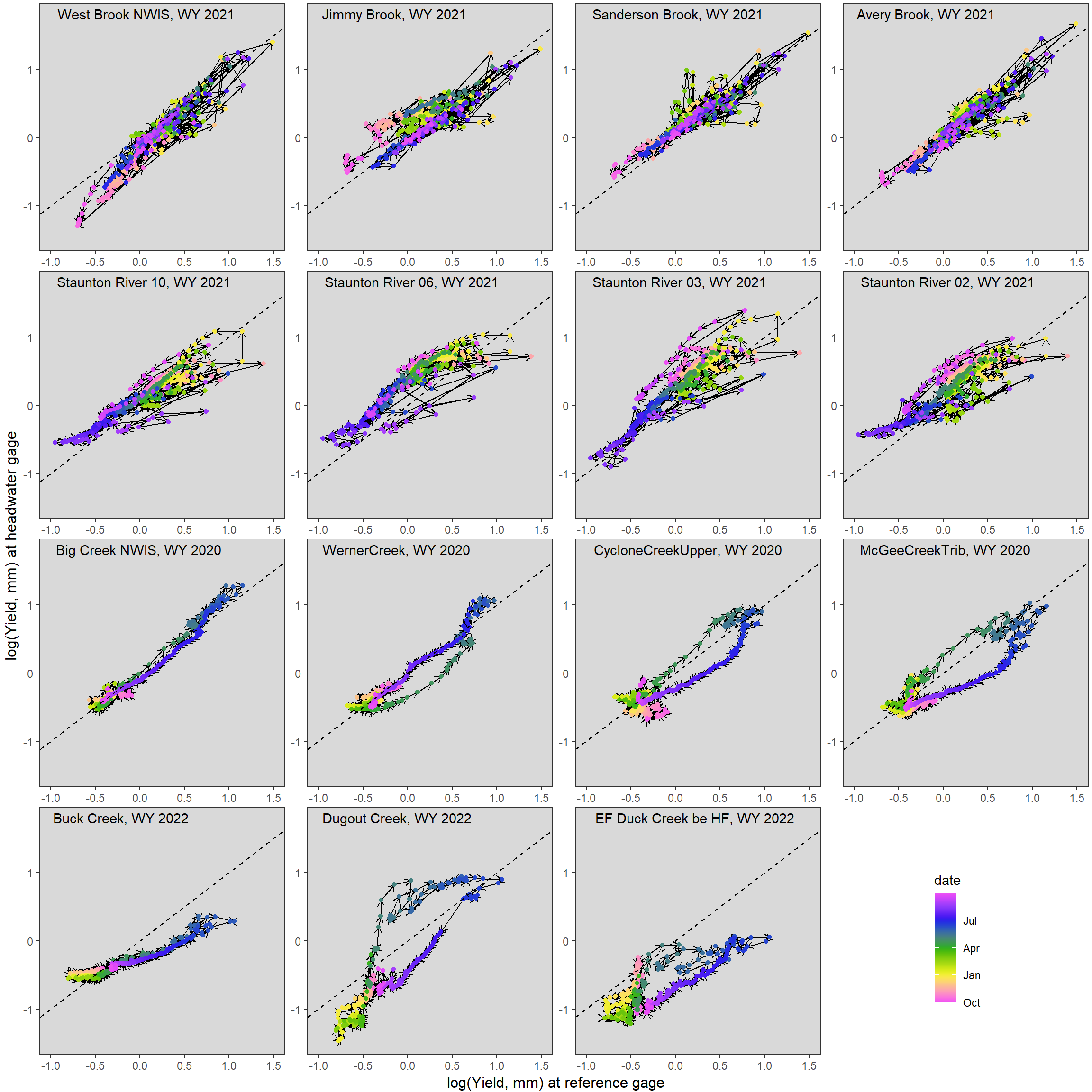

What if we just consider the summer (low flow) period, July - September? In some ways, we see an opposite pattern relative to that describe above. In that we see greater hysteretic behavior in rain-dominated basins (driven by frequent summer storms and lagged runoff response) and less hysteretic behavior in snow-dominated basins, as all streams are in recession from the spring snowmelt peak. However, in general, we see greater divergence from a 1:1 relationship in snowmelt vs rain-dominated basins.

Code

ggarrange(hystplotfunlin(mysite = "West Brook NWIS", wy = 2021, months = c(7:9)) + theme(legend.position = "none"),
          hystplotfunlin(mysite = "Jimmy Brook", wy = 2021, months = c(7:9)) + theme(legend.position = "none"),
          hystplotfunlin(mysite = "Sanderson Brook", wy = 2021, months = c(7:9)) + theme(legend.position = "none"),
          hystplotfunlin(mysite = "Avery Brook", wy = 2021, months = c(7:9)) + theme(legend.position = "none"),
          
          hystplotfunlin(mysite = "Staunton River 10", wy = 2021, months = c(7:9)) + theme(legend.position = "none"),
          hystplotfunlin(mysite = "Staunton River 06", wy = 2021, months = c(7:9)) + theme(legend.position = "none"),
          hystplotfunlin(mysite = "Staunton River 03", wy = 2021, months = c(7:9)) + theme(legend.position = "none"),
          hystplotfunlin(mysite = "Staunton River 02", wy = 2021, months = c(7:9)) + theme(legend.position = "none"),
          
          hystplotfunlin(mysite = "Big Creek NWIS", wy = 2020, months = c(7:9)) + theme(legend.position = "none"),
          hystplotfunlin(mysite = "WernerCreek", wy = 2020, months = c(7:9)) + theme(legend.position = "none"),
          hystplotfunlin(mysite = "CycloneCreekUpper", wy = 2020, months = c(7:9)) + theme(legend.position = "none"),
          hystplotfunlin(mysite = "McGeeCreekTrib", wy = 2020, months = c(7:9)) + theme(legend.position = "none"),
          
          hystplotfunlin(mysite = "Buck Creek", wy = 2022, months = c(7:9)) + theme(legend.position = "none"),
          hystplotfunlin(mysite = "Dugout Creek", wy = 2022, months = c(7:9)) + theme(legend.position = "none"),
          hystplotfunlin(mysite = "EF Duck Creek be HF", wy = 2022, months = c(7:9)) + theme(legend.position = "none"),
          get_legend(hystplotfunlin(mysite = "EF Duck Creek be HF", wy = 2022, months = c(7:9))),
          
          nrow = 4, ncol = 4) %>%
  annotate_figure(left = text_grob("log(Yield, mm) at headwater gage", rot = 90),
                  bottom = text_grob("log(Yield, mm) at reference gage"))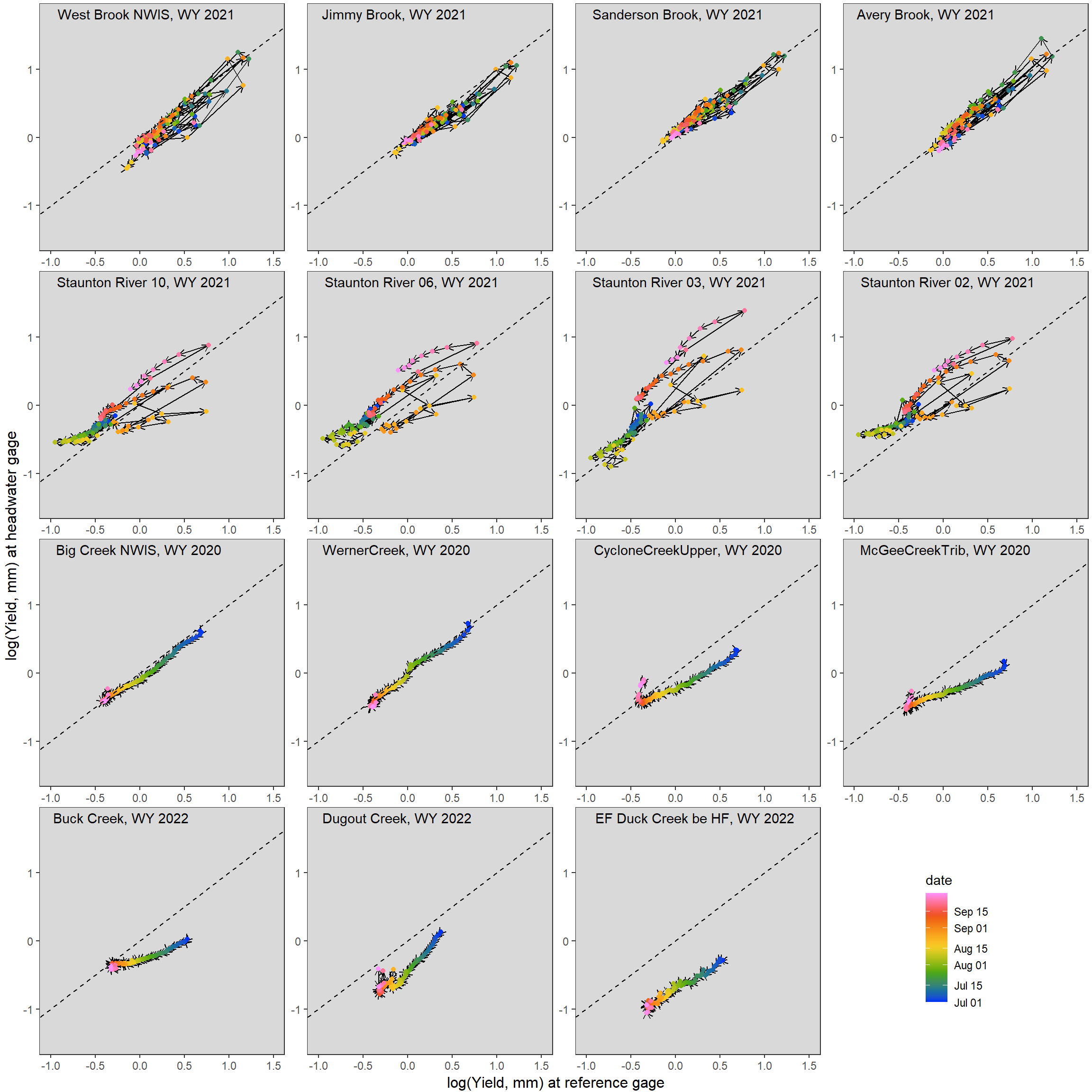

11.3.1 Interactive

11.3.1.1 West Brook

Code

ggplotly(hystplotfun(mysite = "West Brook NWIS", wy = 2021))

Code

ggplotly(hystplotfun(mysite = "Jimmy Brook", wy = 2021))

Code

ggplotly(hystplotfun(mysite = "Sanderson Brook", wy = 2021))

Code

ggplotly(hystplotfun(mysite = "Avery Brook", wy = 2021))

11.3.1.2 Staunton River

Code

ggplotly(hystplotfun(mysite = "Staunton River 10", wy = 2021))

Code

ggplotly(hystplotfun(mysite = "Staunton River 06", wy = 2021))

Code

ggplotly(hystplotfun(mysite = "Staunton River 03", wy = 2021))

Code

ggplotly(hystplotfun(mysite = "Staunton River 02", wy = 2021))

11.3.1.3 Flathead

Code

ggplotly(hystplotfun(mysite = "Big Creek NWIS", wy = 2020))

Code

ggplotly(hystplotfun(mysite = "WernerCreek", wy = 2020))

Code

ggplotly(hystplotfun(mysite = "CycloneCreekUpper", wy = 2020))

Code

ggplotly(hystplotfun(mysite = "McGeeCreekTrib", wy = 2020))

11.3.1.4 Yellowstone

Code

ggplotly(hystplotfun(mysite = "Buck Creek", wy = 2022))

Code

ggplotly(hystplotfun(mysite = "Dugout Creek", wy = 2022))

Code

ggplotly(hystplotfun(mysite = "EF Duck Creek be HF", wy = 2022))

11.4 Frequency and magnitude

Calculate index of hystereis for each event and characterize size-years according the frequency of events and magnitude of hysteretic effects.

Conduct baseflow extraction, event delineation, and calculate event-specific hysteresis index using dynamic time warping (Xue et al. 2024).

Code

# set baseflow extraction and event delineation parameters
alp <- 0.95
numpass <- 3
thresh <- 0.75

# empty list to story site-year data
hysteresis_list <- list()

for (j in 1:nrow(mysiteyrs)) {
  # filter data by site name and water year
  dd <- dat_clean_hyst %>% filter(site_name == mysiteyrs$site_name[j], WaterYear == mysiteyrs$WaterYear[j])
  
  # baseflow extraction on big G yield
  dd <- dd %>% 
    filter(!is.na(Yield_mm_big)) %>% 
    mutate(bf = baseflowB(Yield_mm_big, alpha = alp, passes = numpass)$bf, 
           bfi = baseflowB(Yield_mm_big, alpha = alp, passes = numpass)$bfi) %>%
    ungroup()
  
  # delineate events
  events <- eventBaseflow(dd$Yield_mm_big, BFI_Th = thresh, bfi = dd$bfi)
  events <- events %>% mutate(len = end - srt + 1)
  
  #print("Done - baseflow extraction and event delineation")
  
  ## Tidy events
  # define positions of non-events
  # srt <- c(1)
  # end <- c(events$srt[1]-1)
  # for (i in 2:(dim(events)[1])) {
  #   srt[i] <- events$end[i-1]+1
  #   end[i] <- events$srt[i]-1
  # }
  # nonevents <- data.frame(tibble(srt, end) %>% 
  #                           mutate(len = end - srt) %>% 
  #                           filter(len >= 0) %>% select(-len) %>% 
  #                           add_row(srt = events$end[dim(events)[1]]+1, end = dim(dd)[1])
  #                        )

  # create vectors of binary event/non-event and event IDs
  isevent_vec <- rep(2, times = dim(dd)[1])
  eventid_vec <- rep(NA, times = dim(dd)[1])
  for (i in 1:dim(events)[1]) { 
    isevent_vec[c(events[i,1]:events[i,2])] <- 1 
    eventid_vec[c(events[i,1]:events[i,2])] <- i
  }

  # # create vector of non-event IDs
  # noneventid_vec <- rep(NA, times = dim(dd)[1])
  # for (i in 1:dim(nonevents)[1]) { noneventid_vec[c(nonevents[i,1]:nonevents[i,2])] <- i }
  # 
  # # create vector of "agnostic events": combined hydro events and non-events
  # agnevents <- rbind(events %>% select(srt, end) %>% mutate(event = 1), nonevents %>% mutate(event = 0)) %>% arrange((srt))
  # agneventid_vec <- c()
  # for (i in 1:dim(agnevents)[1]){ agneventid_vec[c(agnevents[i,1]:agnevents[i,2])] <- i }

  # add event/non-event vectors to Big G data
  dd <- dd %>% 
    mutate(isevent = isevent_vec, 
           eventid = eventid_vec,
           #noneventid = noneventid_vec,
           #agneventid = agneventid_vec,
           big_event_yield = ifelse(isevent_vec == 1, Yield_mm_big, NA),
           big_nonevent_yield = ifelse(isevent_vec == 2, Yield_mm_big, NA),
           big_event_quick = big_event_yield - bf) %>%
    rename(big_bf = bf, big_bfi = bfi)
  
  #print("Done - tidy events")
  
  # calculate hysteresis index for each event using dynamic time warping
  event_list <- list()
  for (i in 1:max(dd$eventid, na.rm = TRUE)) {
    # filter by each event and normalized big and little Yield
    ddd <- dd %>% filter(eventid == i, !is.na(logYield), !is.na(logYield_big))
    dddd <- dd %>% filter(date %in% c(min(ddd$date)-1, max(ddd$date)+1))
    ddd <- ddd %>% 
      bind_rows(dddd) %>% 
      arrange(date) %>% 
      mutate(weight = (logYield_big - min(logYield_big)) / (max(logYield_big) - min(logYield_big)),
             yield_little_norm = (logYield - min(logYield)) / (max(logYield) - min(logYield)),
             yield_big_norm = (logYield_big - min(logYield_big)) / (max(logYield_big) - min(logYield_big)))
    # ddd %>%
    #   ggplot(aes(x = yield_big_norm, y = yield_little_norm, color = date)) +
    #   geom_segment(aes(xend = c(tail(yield_big_norm, n = -1), NA), yend = c(tail(yield_little_norm, n = -1), NA)), 
    #                arrow = arrow(length = unit(0.2, "cm")), color = "black") +
    #   geom_point() + 
    #   geom_abline(intercept = 0, slope = 1, linetype = "dashed") + 
    #   scale_color_gradientn(colors = cet_pal(250, name = "r1"), trans = "date") +
    #   theme_bw() + 
    #   theme(panel.grid.major = element_blank(), panel.grid.minor = element_blank())
  
    # align data using dynamic time warping, allow for error handling (e.g., skips if either big or little g is constant during event, b/c normalization returns NaN)
    skip_to_next <- FALSE
    tryCatch(align <- dtw(x = unlist(ddd %>% select(yield_big_norm)), y = unlist(ddd %>% select(yield_little_norm)), step = asymmetric, keep = TRUE), error = function(e) { skip_to_next <<- TRUE })
    if(skip_to_next) { next }
    #align <- dtw(x = unlist(ddd %>% select(yield_big_norm)), y = unlist(ddd %>% select(yield_little_norm)), step = asymmetric, keep = TRUE)
    # plot(align, type = "threeway")
    # plot(align, type = "twoway", offset = -1)
  
    # find time-warped distance, S_i in Xue et al. (2024)
    ddd <- ddd %>% mutate(distance = align$index1 - align$index2)
    # ddd %>% 
    #   ggplot(aes(x = date, y = distance*weight)) + 
    #   geom_bar(stat = "identity") +
    #   theme_bw()
  
    # summarize event
    event_list[[i]] <- ddd %>% 
      group_by(site_name, basin, subbasin, region, WaterYear) %>%
      summarize(eventdays = n(),
                eventid = i,
                mindate = min(date),
                maxdate = max(date),
                totalyieldevent_little = sum(Yield_mm),
                totalyieldevent_big = sum(Yield_mm_big),
                hysteresis = sum(ddd$weight * ddd$distance) / sum(ddd$weight) # hysteresis index as in Xue et al (2024)
                ) %>%
      ungroup()
  }
  #print("Done - dynamic time warping")
  hysteresis_list[[j]] <- do.call(bind_rows, event_list)
  print(j)
}

# bind to tibble
hysteresis <- do.call(bind_rows, hysteresis_list) %>% 
  left_join(mysiteyrs %>% select(site_name, basin, subbasin, region, WaterYear, numdays, totalyield_site)) %>%
  mutate(propyield = totalyieldevent_little / totalyield_site)

# write to file
write_csv(hysteresis, "C:/Users/jbaldock/OneDrive - DOI/Documents/USGS/EcoDrought/EcoDrought Working/EcoDrought-Analysis/Qualitative/hysteresis.csv")

Load hysteresis file

Code

hysteresis <- read_csv("C:/Users/jbaldock/OneDrive - DOI/Documents/USGS/EcoDrought/EcoDrought Working/EcoDrought-Analysis/Qualitative/hysteresis.csv")
# hysteresis <- hysteresis %>% 
#   group_by(subbasin, WaterYear) %>%
#   mutate(eventid = as.numeric(as.factor(mindate))) %>%
#   ungroup()

11.4.1 Visualize hysteresis

Distribution of hystersis index by subbasin

Code

hysteresis %>%
  ggplot(aes(x = subbasin, y = hysteresis, fill = subbasin)) + 
  geom_boxplot(outlier.shape = NA) + 
  geom_jitter(height = 0, width = 0.25, alpha = 0.2) +
  xlab("Sub-basin") + ylab("Xue hysteresis index") +
  theme_bw() + 
  theme(panel.grid.major = element_blank(), panel.grid.minor = element_blank(),
        axis.text.x = element_text(angle = 45, vjust = 0.5, hjust = 0.4))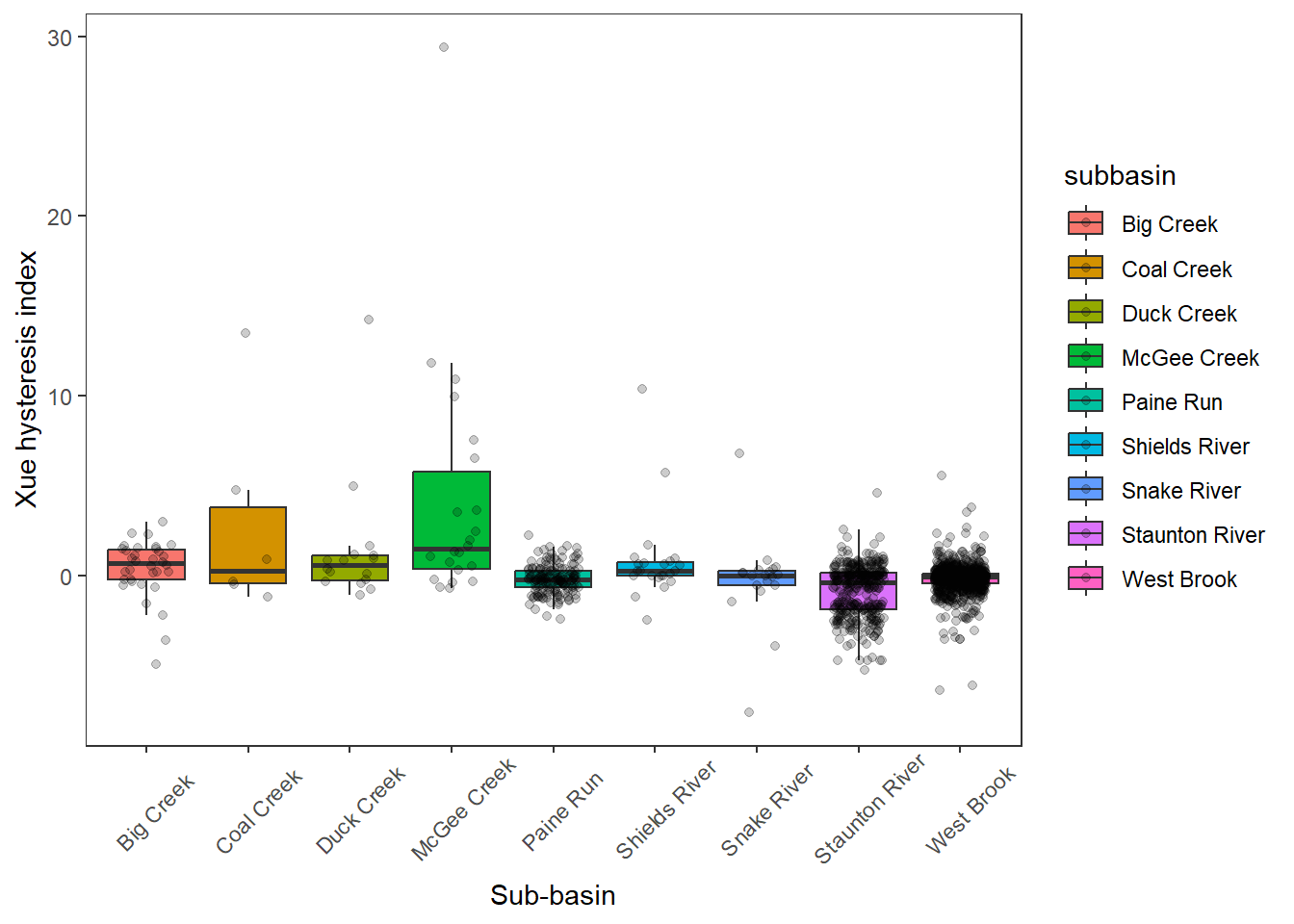

Magnitude of hysteresis by length of event

Code

hysteresis %>%
  ggplot(aes(x = eventdays, y = abs(hysteresis), color = subbasin)) + 
  geom_point() +
  xlab("Event length (days)") + ylab("Xue hysteresis index (absolute value)") +
  theme_bw() + 
  theme(panel.grid.major = element_blank(), panel.grid.minor = element_blank())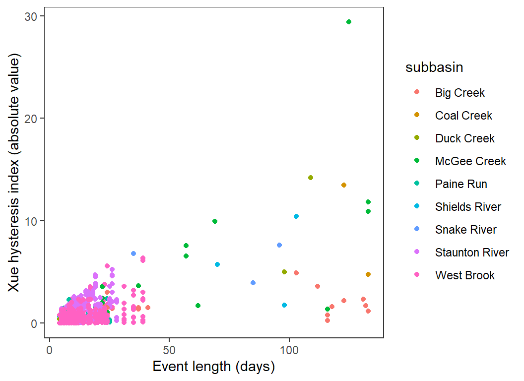

Magnitude of hysteresis by length of event, by subbasin and site

Code

hysteresis %>%
  #filter(eventdays >= 6) %>%
  ggplot(aes(x = eventdays, y = abs(hysteresis), color = site_name, group = site_name)) + 
  geom_point() +
  geom_smooth(method = "lm") +
  facet_wrap(~subbasin, scales = "free") +
  xlab("Event length (days)") + ylab("Xue hysteresis index (absolute value)") +
  theme_bw() + 
  theme(panel.grid.major = element_blank(), panel.grid.minor = element_blank(), legend.position = "none")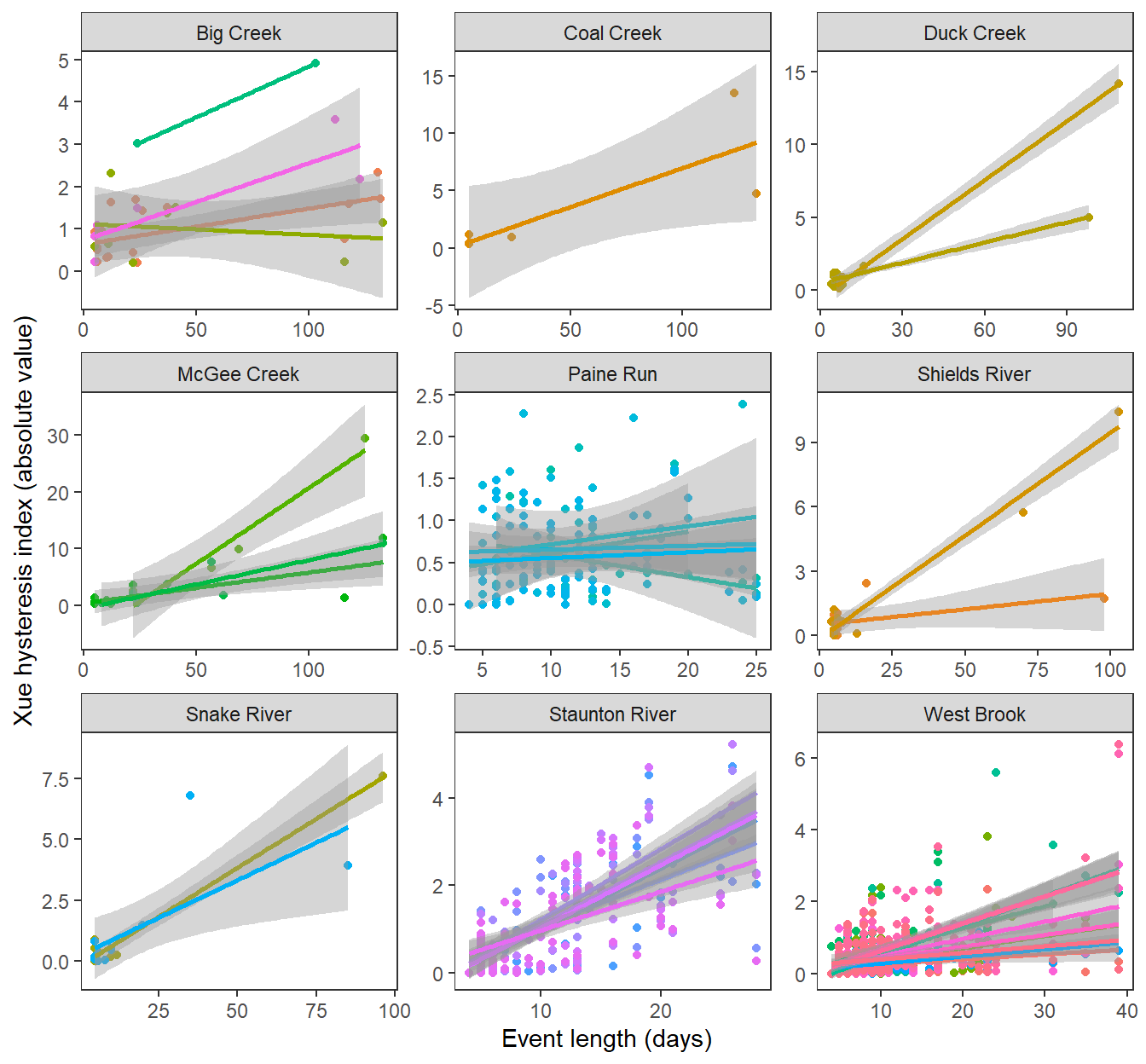

Magnitude of hysteresis by proportion of annual yield in event

Code

hysteresis %>%
  ggplot(aes(x = propyield, y = abs(hysteresis), color = subbasin)) + 
  geom_point() +
  xlab("Proportion of annual yield in event") + ylab("Xue hysteresis index (absolute value)") +
  theme_bw() + 
  theme(panel.grid.major = element_blank(), panel.grid.minor = element_blank())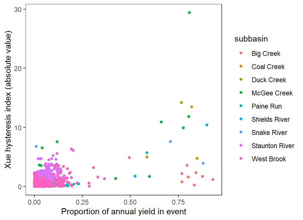

Magnitude of hysteresis by proportion of annual yield in event, by subbasin and site

Code

hysteresis %>%
  ggplot(aes(x = propyield, y = abs(hysteresis), color = site_name, group = site_name)) + 
  geom_point() +
  geom_smooth(method = "lm") +
  facet_wrap(~subbasin, scales = "free") +
  xlab("Proportion of annual yield in event") + ylab("Xue hysteresis index (absolute value)") +
  theme_bw() + 
  theme(panel.grid.major = element_blank(), panel.grid.minor = element_blank(), legend.position = "none")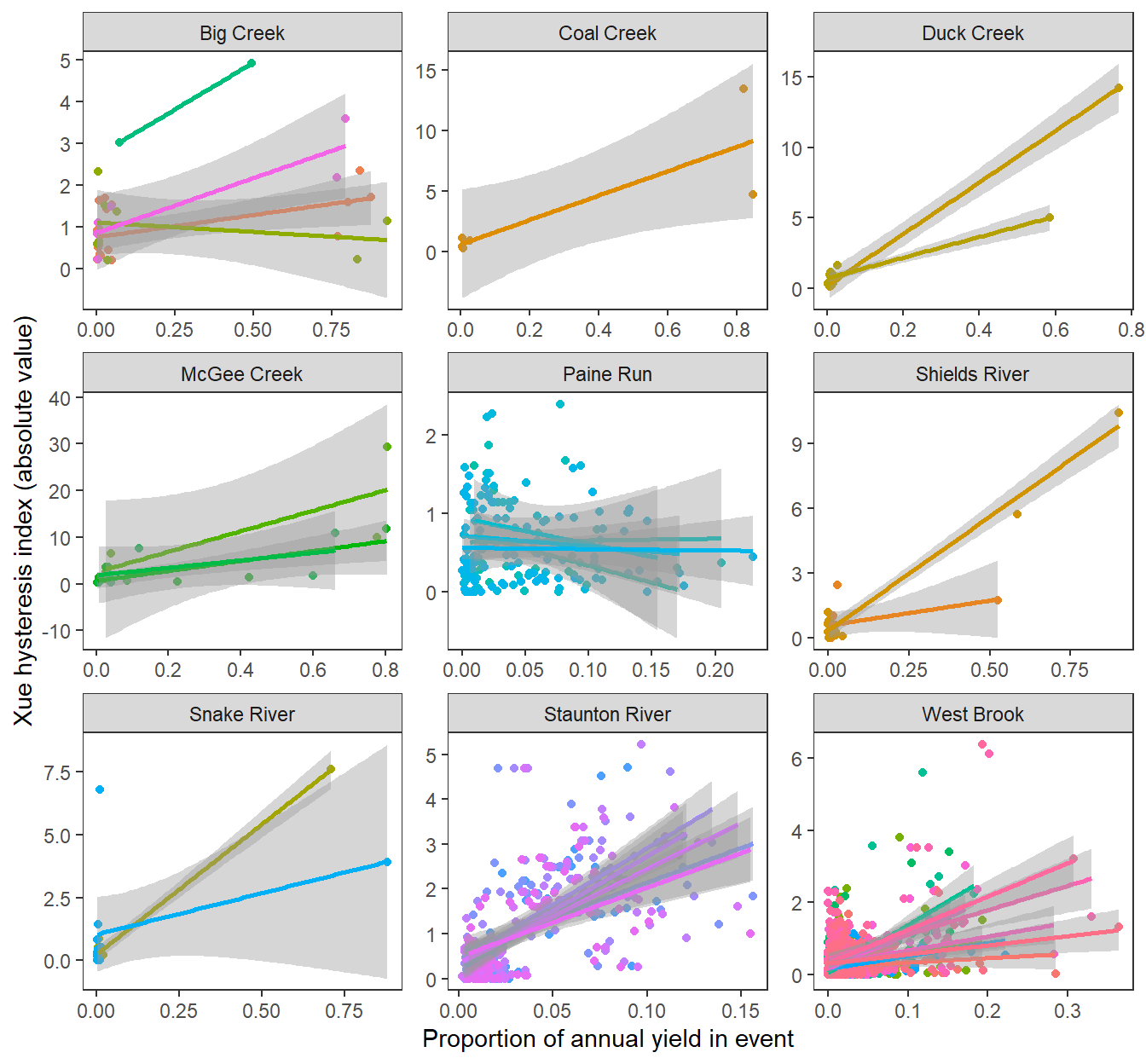

11.4.2 Site-year summary

Characterize site-years along axes of mean annual event duration/magnitude and magnitude of hysteres.

Summarize hysteresis by site and year

Code

temp <- hysteresis %>% 
  group_by(subbasin, site_name, WaterYear) %>% 
  summarize(freq = n(), 
            meanpropyield = mean(propyield),
            meanhyst = mean(abs(hysteresis))) %>%
  mutate(logmeanhyst = log(meanhyst)) %>%
  ungroup() 
temp

# A tibble: 87 × 7
   subbasin   site_name       WaterYear  freq meanpropyield meanhyst logmeanhyst
   <chr>      <chr>               <dbl> <int>         <dbl>    <dbl>       <dbl>
 1 Big Creek  Big Creek NWIS       2019     2         0.435    2.02       0.703 
 2 Big Creek  Big Creek NWIS       2020     3         0.294    0.954     -0.0473
 3 Big Creek  Big Creek NWIS       2021     6         0.143    0.878     -0.130 
 4 Big Creek  Big Creek NWIS       2022     7         0.134    0.746     -0.294 
 5 Big Creek  Hallowat Creek…      2020     2         0.465    0.868     -0.141 
 6 Big Creek  Hallowat Creek…      2022     6         0.162    1.05       0.0452
 7 Big Creek  NicolaCreek          2019     2         0.284    3.96       1.38  
 8 Big Creek  WernerCreek          2019     2         0.407    1.84       0.608 
 9 Big Creek  WernerCreek          2020     4         0.202    1.43       0.358 
10 Coal Creek CycloneCreekUp…      2019     2         0.436    2.84       1.04  
# ℹ 77 more rows

Characterize sites/subbasins along axes of event frequency and magnitude (mean annual proportion of flow within event).

Code

hull <- temp %>% group_by(subbasin) %>% slice(chull(freq, meanpropyield))
temp %>%
  ggplot(aes(x = freq, y = meanpropyield)) + 
  #geom_polygon(data = hull, aes(fill = subbasin), alpha = 0.5) +
  #geom_smooth(color = "black", method = "lm") +
  geom_point(aes(color = subbasin)) + 
  xlab("Events per year") + ylab("Proportion of annual yield in event (mean over events)") +
  theme_bw() + 
  theme(panel.grid.major = element_blank(), panel.grid.minor = element_blank())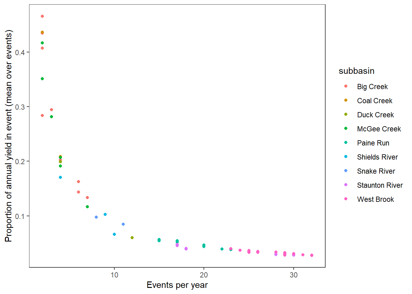

Plot the mean annual magnitude (absolute value) of event-specific hysteresis by event frequency (events per year), with LOESS smoothing.

Code

p1 <- temp %>%
  ggplot(aes(x = freq, y = (meanhyst))) + 
  geom_smooth(color = "black") +
  #geom_smooth(color = "black", method = "glm", formula = y~x, method.args = list(family = gaussian(link = 'log'))) +
  geom_point(aes(color = subbasin)) + 
  xlab("Events per year") + ylab("Mean annual magnitude of hysteresis") +
  theme_bw() + 
  theme(panel.grid.major = element_blank(), panel.grid.minor = element_blank())
p2 <- temp %>%
  ggplot(aes(x = meanpropyield, y = (meanhyst))) + 
  geom_smooth(color = "black") +
  #geom_smooth(color = "black", method = "glm", formula = y~x, method.args = list(family = gaussian(link = 'log'))) +
  geom_point(aes(color = subbasin)) + 
  xlab("Proportion of annual yield in event") + ylab("Mean annual magnitude of hysteresis") +
  theme_bw() + 
  theme(panel.grid.major = element_blank(), panel.grid.minor = element_blank())
ggarrange(p1, p2, nrow = 1, common.legend = TRUE, legend = "right")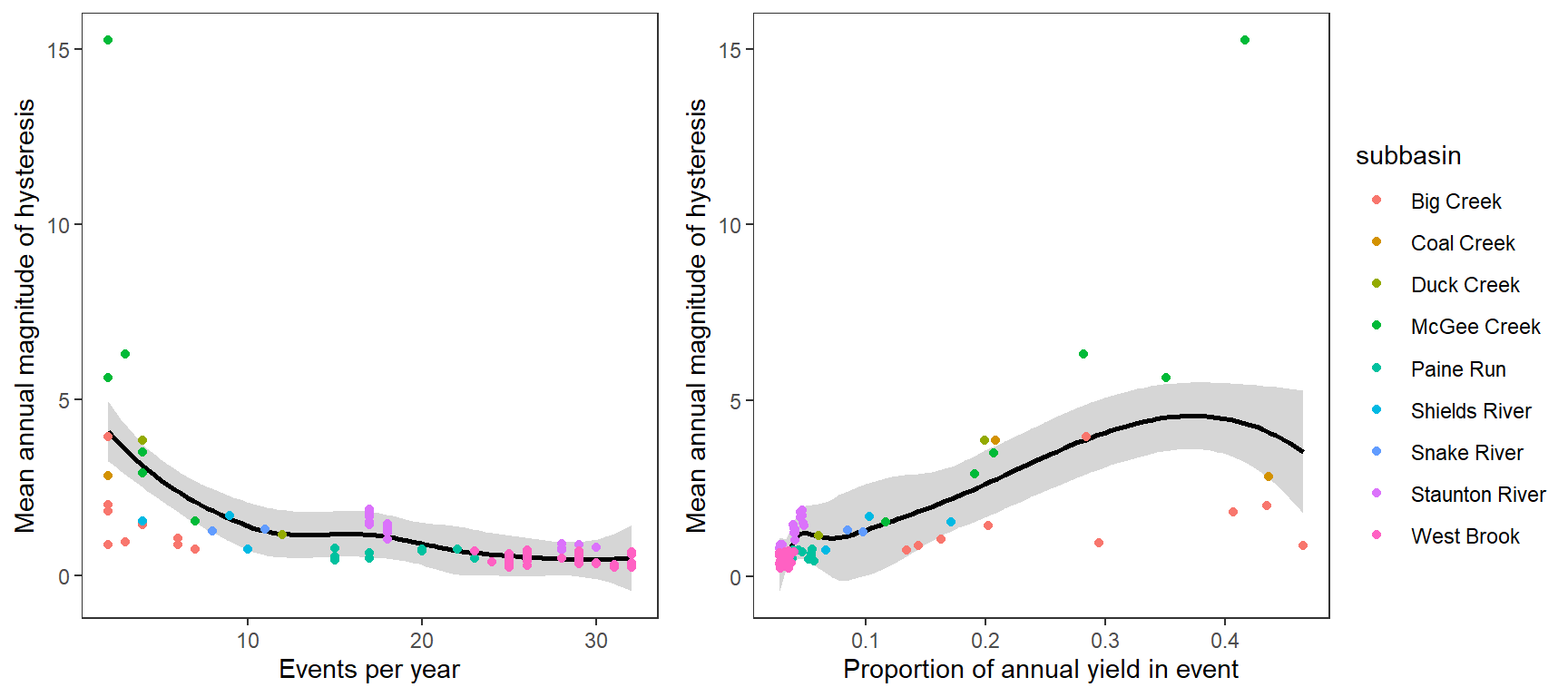

Same as above but plot on log scale (magnitude):

Code

p1 <- temp %>%
  ggplot(aes(x = freq, y = logmeanhyst)) + 
  geom_smooth(color = "black", method = "lm") +
  geom_point(aes(color = subbasin)) + 
  xlab("Events per year") + ylab("(log) Mean annual magnitude of hysteresis") +
  theme_bw() + 
  theme(panel.grid.major = element_blank(), panel.grid.minor = element_blank())
p2 <- temp %>%
  ggplot(aes(x = meanpropyield, y = logmeanhyst)) + 
  geom_smooth(color = "black", method = "lm") +
  geom_point(aes(color = subbasin)) + 
  xlab("Proportion of annual yield in event") + ylab("(log) Mean annual magnitude of hysteresis") +
  theme_bw() + 
  theme(panel.grid.major = element_blank(), panel.grid.minor = element_blank())
ggarrange(p1, p2, nrow = 1, common.legend = TRUE, legend = "right")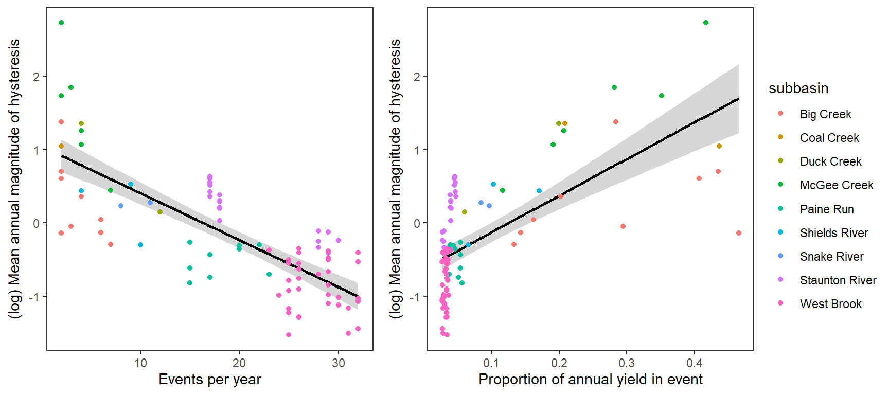

Replace regression line with convex hulls

Code

hull <- temp %>% group_by(subbasin) %>% slice(chull(freq, logmeanhyst))
p1 <- temp %>%
  ggplot(aes(x = freq, y = logmeanhyst)) + 
  geom_polygon(data = hull, aes(fill = subbasin), alpha = 0.4) +
  geom_point(aes(color = subbasin)) + 
  xlab("Events per year") + ylab("(log) Mean annual magnitude of hysteresis") +
  theme_bw() + 
  theme(panel.grid.major = element_blank(), panel.grid.minor = element_blank())
hull <- temp %>% group_by(subbasin) %>% slice(chull(meanpropyield, logmeanhyst))
p2 <- temp %>%
  ggplot(aes(x = meanpropyield, y = logmeanhyst)) + 
  geom_polygon(data = hull, aes(fill = subbasin), alpha = 0.4) +
  geom_point(aes(color = subbasin)) + 
  xlab("Proportion of annual yield in event") + ylab("(log) Mean annual magnitude of hysteresis") +
  theme_bw() + 
  theme(panel.grid.major = element_blank(), panel.grid.minor = element_blank())
ggarrange(p1, p2, nrow = 1, common.legend = TRUE, legend = "right")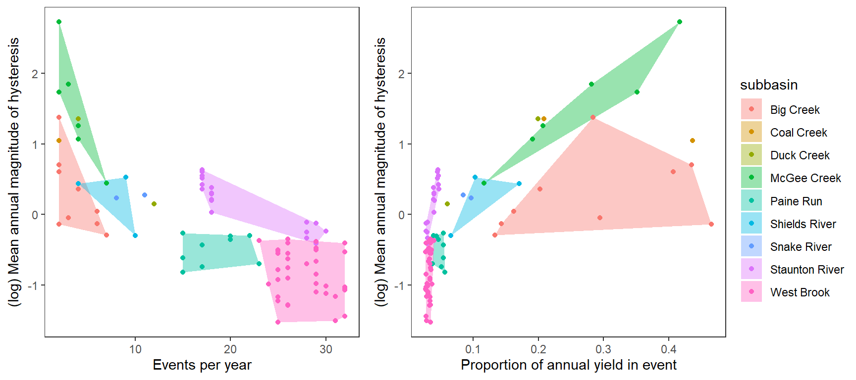

Alternatively, plot frequency by magnitude and with point color/size. I don’t think this tells the story as well as the convex hull plots.

Code

p1 <- temp %>%
  ggplot(aes(x = meanpropyield, y = freq)) + 
  # geom_polygon(data = hull, aes(fill = subbasin), alpha = 0.5) +
  geom_point(aes(color = subbasin, size = logmeanhyst)) + 
  scale_size_continuous(range = c(0.1,5)) +
  xlab("Proportion of annual yield in event") + ylab("Events per year") +
  theme_bw() + 
  theme(panel.grid.major = element_blank(), panel.grid.minor = element_blank())

p2 <- temp %>%
  ggplot(aes(x = meanpropyield, y = freq)) + 
  # geom_polygon(data = hull, aes(fill = subbasin), alpha = 0.5) +
  geom_point(aes(color = logmeanhyst), size = 2) + 
  xlab("Proportion of annual yield in event") + ylab("Events per year") +
  theme_bw() + 
  theme(panel.grid.major = element_blank(), panel.grid.minor = element_blank())

ggarrange(p1, p2, nrow = 1)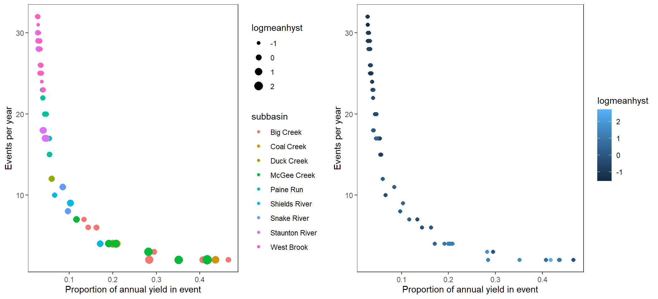

11.5 By event

Code

mycols <- c(brewer.pal(8, "Dark2"), "dodgerblue", "darkorchid")

events <- hysteresis %>% filter(subbasin == "Staunton River", WaterYear == 2020, eventid == 2)
length(unique(events$mindate))

[1] 1

Code

length(unique(events$maxdate))

[1] 1

Code

dat_clean_hyst %>% 
  filter(subbasin == unique(events$subbasin), 
         date >= unique(events$mindate), 
         date <= unique(events$maxdate)) %>%
  ggplot(aes(x = logYield_big, y = logYield, group = site_name, color = site_name)) +
  geom_segment(aes(xend = c(tail(logYield_big, n = -1), NA), yend = c(tail(logYield, n = -1), NA)), 
               arrow = arrow(length = unit(0.2, "cm")), color = "black") +
  geom_point() + 
  geom_abline(intercept = 0, slope = 1, linetype = "dashed") + 
  #scale_color_gradientn(colors = cet_pal(250, name = "r1"), trans = "date") +
  theme_bw() + 
  theme(panel.grid.major = element_blank(), panel.grid.minor = element_blank())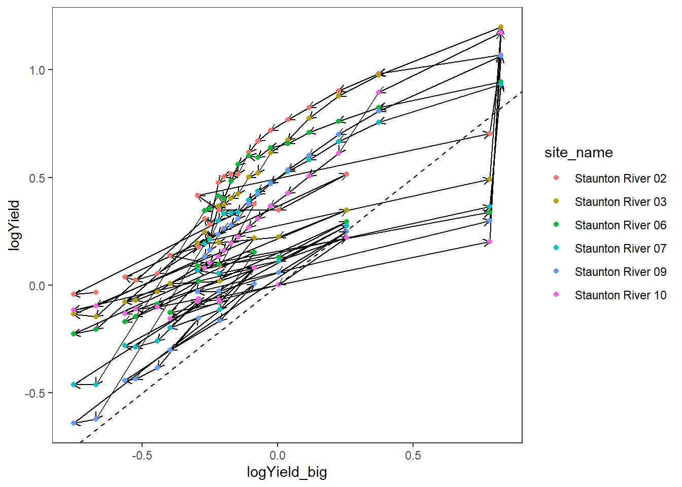

Code

dat_clean_hyst %>% 
  filter(subbasin == unique(events$subbasin), 
         date >= unique(events$mindate), 
         date <= unique(events$maxdate)) %>%
  ggplot(aes(x = logYield_big, y = logYield, group = site_name, color = site_name)) +
  geom_segment(aes(xend = c(tail(logYield_big, n = -1), NA), yend = c(tail(logYield, n = -1), NA)), 
               arrow = arrow(length = unit(0.2, "cm")), color = "black") +
  geom_point() + 
  geom_abline(intercept = 0, slope = 1, linetype = "dashed") + 
  #scale_color_gradientn(colors = cet_pal(250, name = "r1"), trans = "date") +
  facet_wrap(~site_name) +
  theme_bw() + 
  theme(panel.grid.major = element_blank(), panel.grid.minor = element_blank(), legend.position = "none")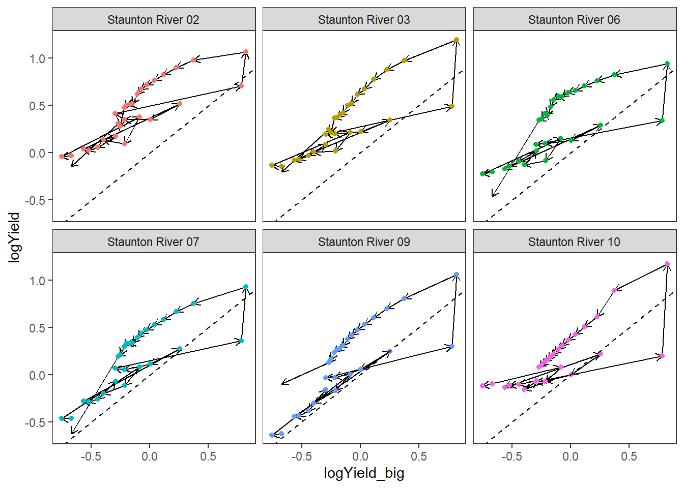

Code

temp2 <- hysteresis %>% 
  #filter(subbasin == "West Brook") %>%
  mutate(eventid_global = paste(WaterYear, eventid, sep = "-")) %>%
  group_by(subbasin, eventid_global, mindate, totalyieldevent_big) %>%
  summarize(nsites = n(), sdhyst = sd(hysteresis), meanhyst = mean(abs(hysteresis)), sd_totalyieldevent_little = sd(totalyieldevent_little)) %>%
  ungroup()

temp2$antecedant <- NA
for (i in 1:dim(temp2)[1]) {
  temp2$antecedant[i] <- sum(unlist(dat_clean_big %>% filter(subbasin == unique(temp2$subbasin), date < temp2$mindate[i], date >= temp2$mindate[i]-days(30)) %>% select(Yield_mm)))
}
head(temp2)

# A tibble: 6 × 9
  subbasin  eventid_global mindate    totalyieldevent_big nsites sdhyst meanhyst
  <chr>     <chr>          <date>                   <dbl>  <int>  <dbl>    <dbl>
1 Big Creek 2019-1         2018-10-26               14.9       3  0.815    2.08 
2 Big Creek 2019-2         2019-03-21              188.        1 NA        4.91 
3 Big Creek 2019-2         2019-03-21              291.        1 NA        2.18 
4 Big Creek 2019-2         2019-03-21              352.        1 NA        1.77 
5 Big Creek 2020-1         2019-12-21                2.38      3  0.355    0.937
6 Big Creek 2020-2         2020-01-31                2.19      2  0        0.226
# ℹ 2 more variables: sd_totalyieldevent_little <dbl>, antecedant <dbl>

Larger events at big G (cumulative flow) tend to be associated with larger events at little g’s.

Code

hysteresis %>% #filter(subbasin == "West Brook") %>%
  mutate(eventid_global = paste(WaterYear, eventid, sep = "-")) %>%
  ggplot(aes(x = totalyieldevent_big, y = totalyieldevent_little)) + 
  geom_point(aes(color = eventid_global)) +
  geom_abline(intercept = 0, slope = 1, linetype = "dashed") +
  geom_quantile(color = "black") +
  theme_bw() + theme(panel.grid.major = element_blank(), panel.grid.minor = element_blank(), legend.position = "none") +
  facet_wrap(~subbasin, scales = "free")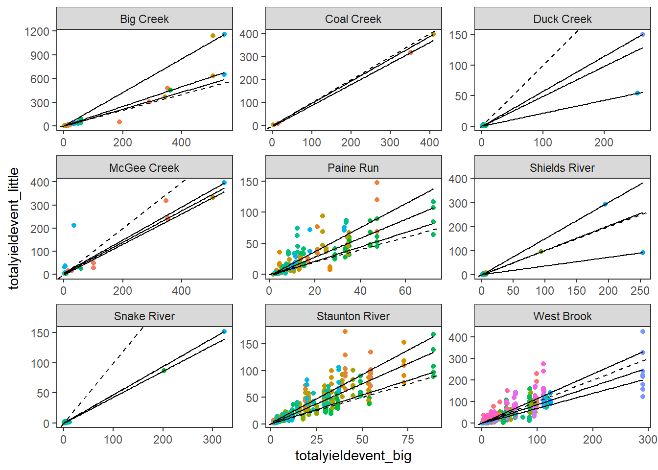

Variation among little g flow volume also increases with event magnitude.

Code

temp2 %>%
  ggplot(aes(x = log(totalyieldevent_big), y = log(sd_totalyieldevent_little))) +
  geom_point() +
  geom_smooth(method = "lm") +
  xlab("(log) Cumulative yield at big G") + ylab("(log) SD cumulative yield at little G") +
  theme_bw() + theme(panel.grid.major = element_blank(), panel.grid.minor = element_blank(), legend.position = "none") +
  facet_wrap(~subbasin, scales = "free")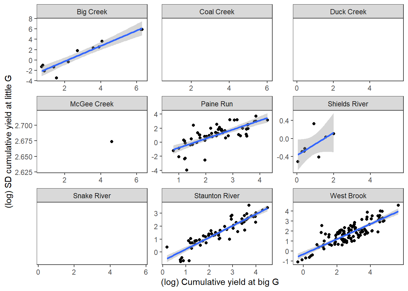

Events with greater average hysteresis also tend to be more variable among the little g’s

Code

p1 <- temp2 %>%
  ggplot(aes(x = meanhyst, y = sdhyst)) +
  geom_point() +
  geom_smooth(method = "lm") +
  xlab("Mean hysteresis (among little g's)") + ylab("SD hysteresis (among little g's)") +
  theme_bw() + theme(panel.grid.major = element_blank(), panel.grid.minor = element_blank(), legend.position = "none")

p2 <- temp2 %>%
  ggplot(aes(x = log(meanhyst), y = log(sdhyst))) +
  geom_point() +
  geom_smooth(method = "lm") +
  xlab("(log) Mean hysteresis (among little g's)") + ylab("(log) SD hysteresis (among little g's)") +
  theme_bw() + theme(panel.grid.major = element_blank(), panel.grid.minor = element_blank(), legend.position = "none")

ggarrange(p1, p2, ncol = 2)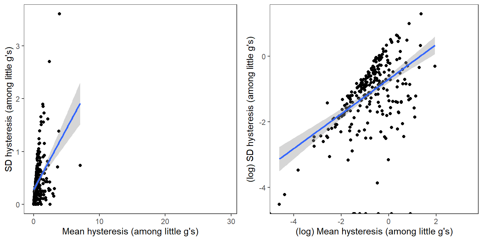

Generally, larger events (cumulative yield at big G) lead to greater mean hysteresis among little g’s and more variation in hysteresis among little g’s

Code

p1 <- temp2 %>%
  filter(sdhyst > 0) %>%
  ggplot(aes(x = (totalyieldevent_big), y = (meanhyst))) +
  geom_point() +
  geom_smooth() +
  xlab("Cumulative yield at big G") + ylab("Mean hysteresis") +
  theme_bw() + theme(panel.grid.major = element_blank(), panel.grid.minor = element_blank(), legend.position = "none")

p2 <- temp2 %>%
  filter(sdhyst > 0) %>%
  ggplot(aes(x = (totalyieldevent_big), y = (sdhyst))) +
  geom_point() +
  geom_smooth() +
  xlab("Cumulative yield at big G") + ylab("SD hysteresis)") +
  theme_bw() + theme(panel.grid.major = element_blank(), panel.grid.minor = element_blank(), legend.position = "none")

p3 <- temp2 %>%
  filter(sdhyst > 0) %>%
  ggplot(aes(x = log(totalyieldevent_big), y = log(meanhyst))) +
  geom_point() +
  geom_smooth(method = "lm") +
  xlab("(log) Cumulative yield at big G") + ylab("(log) Mean hysteresis") +
  theme_bw() + theme(panel.grid.major = element_blank(), panel.grid.minor = element_blank(), legend.position = "none")

p4 <- temp2 %>%
  filter(sdhyst > 0) %>%
  ggplot(aes(x = log(totalyieldevent_big), y = log(sdhyst))) +
  geom_point() +
  geom_smooth(method = "lm") +
  xlab("(log) Cumulative yield at big G") + ylab("(log) SD hysteresis") +
  theme_bw() + theme(panel.grid.major = element_blank(), panel.grid.minor = element_blank(), legend.position = "none")

ggarrange(p1, p2, p3, p4, nrow = 2, ncol = 2)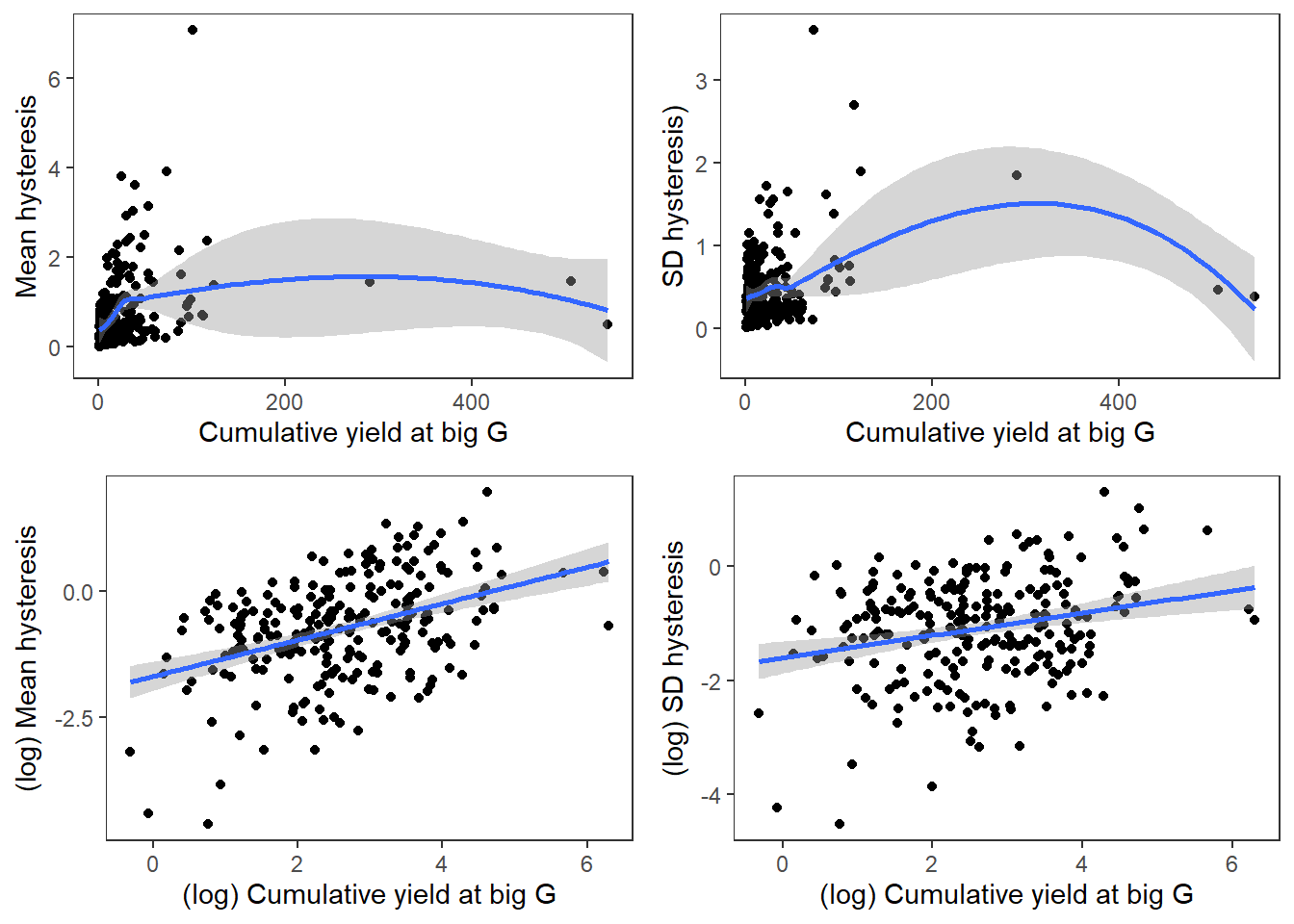

Events with greater average hysteresis also tend to be more variable among the little g’s

Code

p1 <- temp2 %>%
  ggplot(aes(x = antecedant, y = meanhyst)) +
  geom_point() +
  geom_smooth(method = "lm") +
  xlab("Antecedant cumulative flow (30 days)") + ylab("Mean hysteresis") +
  theme_bw() + theme(panel.grid.major = element_blank(), panel.grid.minor = element_blank(), legend.position = "none")

p2 <- temp2 %>%
  ggplot(aes(x = antecedant, y = sdhyst)) +
  geom_point() +
  geom_smooth(method = "lm") +
  xlab("Antecedant cumulative flow (30 days)") + ylab("SD hysteresis") +
  theme_bw() + theme(panel.grid.major = element_blank(), panel.grid.minor = element_blank(), legend.position = "none")

ggarrange(p1, p2, ncol = 2)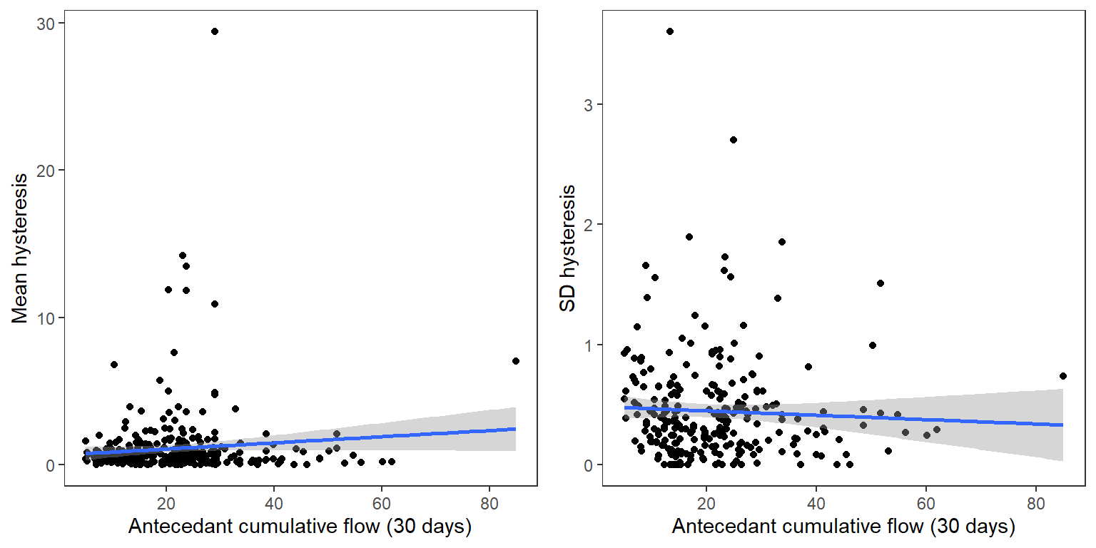

11.6 Test pit

Conduct baseflow separation, event delineation, and dynamic time warping as above, but only for a single site year. For troubleshooting and data visualization

Set parameters and site-year

Code

alp <- 0.95
numpass <- 3
thresh <- 0.75
dd <- dat_clean_hyst %>% filter(site_name == "McGeeCreekLower", WaterYear == 2019)

baseflow separation

Code

dd <- dd %>% 
  filter(!is.na(Yield_mm_big)) %>% 
  mutate(bf = baseflowB(Yield_mm_big, alpha = alp, passes = numpass)$bf, 
         bfi = baseflowB(Yield_mm_big, alpha = alp, passes = numpass)$bfi) %>%
  ungroup()
head(dd)

Event delineation

Code

events <- eventBaseflow(dd$Yield_mm_big, BFI_Th = thresh, bfi = dd$bfi)
events <- events %>% mutate(len = end - srt + 1)
(events)

Tidy events: now add variables to the Big G time series data specifying events and non-events

Code

# define positions of non-events
srt <- c(1)
end <- c(events$srt[1]-1)
for (i in 2:(dim(events)[1])) {
  srt[i] <- events$end[i-1]+1
  end[i] <- events$srt[i]-1
}
nonevents <- data.frame(tibble(srt, end) %>% mutate(len = end - srt) %>% filter(len >= 0) %>% select(-len) %>% add_row(srt = events$end[dim(events)[1]]+1, end = dim(dd)[1]))

# create vectors of binary event/non-event and event IDs
isevent_vec <- rep(2, times = dim(dd)[1])
eventid_vec <- rep(NA, times = dim(dd)[1])
for (i in 1:dim(events)[1]) { 
  isevent_vec[c(events[i,1]:events[i,2])] <- 1 
  eventid_vec[c(events[i,1]:events[i,2])] <- i
}

# create vector of non-event IDs
noneventid_vec <- rep(NA, times = dim(dd)[1])
for (i in 1:dim(nonevents)[1]) { noneventid_vec[c(nonevents[i,1]:nonevents[i,2])] <- i }

# create vector of "agnostic events": combined hydro events and non-events
agnevents <- rbind(events %>% select(srt, end) %>% mutate(event = 1), nonevents %>% mutate(event = 0)) %>% arrange((srt))
agneventid_vec <- c()
for (i in 1:dim(agnevents)[1]){ agneventid_vec[c(agnevents[i,1]:agnevents[i,2])] <- i }

# add event/non-event vectors to Big G data
dd <- dd %>% 
  mutate(isevent = isevent_vec, 
         eventid = eventid_vec,
         noneventid = noneventid_vec,
         agneventid = agneventid_vec,
         big_event_yield = ifelse(isevent_vec == 1, Yield_mm_big, NA),
         big_nonevent_yield = ifelse(isevent_vec == 2, Yield_mm_big, NA),
         big_event_quick = big_event_yield - bf) %>%
  rename(big_bf = bf, big_bfi = bfi)
(dd)

View time series data with Big G event delineation

Code

dd %>% select(date, Yield_mm_big, Yield_mm, big_event_yield, big_nonevent_yield) %>% dygraph() %>% dyRangeSelector() %>% dyAxis("y", label = "Yield (mm)") %>% dyOptions(fillGraph = TRUE, drawGrid = FALSE, axisLineWidth = 1.5)

View hysteresis loops: g~G

Code

dd %>%
  filter(isevent == 1) %>%
  ggplot(aes(x = logYield_big, y = logYield, color = date)) +
  geom_segment(aes(xend = c(tail(logYield_big, n = -1), NA), yend = c(tail(logYield, n = -1), NA)), 
               arrow = arrow(length = unit(0.2, "cm")), color = "black") +
  geom_point() + 
  geom_abline(intercept = 0, slope = 1, linetype = "dashed") + 
  scale_color_gradientn(colors = cet_pal(250, name = "r1"), trans = "date") + 
  facet_wrap(~eventid) +
  theme_bw() + 
  theme(panel.grid.major = element_blank(), panel.grid.minor = element_blank())

Select and view specific event and normalize data

Code

ddd <- dd %>% filter(eventid == 1, !is.na(logYield), !is.na(logYield_big))
dddd <- dd %>% filter(date %in% c(min(ddd$date)-1, max(ddd$date)+1))
ddd <- ddd %>% 
  bind_rows(dddd) %>% 
  arrange(date) %>% 
  mutate(weight = (logYield_big - min(logYield_big, na.rm = TRUE)) / (max(logYield_big, na.rm = TRUE) - min(logYield_big, na.rm = TRUE)),
         yield_little_norm = (logYield - min(logYield, na.rm = TRUE)) / (max(logYield, na.rm = TRUE) - min(logYield, na.rm = TRUE)),
         yield_big_norm = (logYield_big - min(logYield_big, na.rm = TRUE)) / (max(logYield_big, na.rm = TRUE) - min(logYield_big, na.rm = TRUE)))

ddd %>%
  ggplot(aes(x = yield_big_norm, y = yield_little_norm, color = date)) +
  geom_segment(aes(xend = c(tail(yield_big_norm, n = -1), NA), yend = c(tail(yield_little_norm, n = -1), NA)), 
               arrow = arrow(length = unit(0.2, "cm")), color = "black") +
  geom_point() + 
  geom_abline(intercept = 0, slope = 1, linetype = "dashed") + 
  scale_color_gradientn(colors = cet_pal(250, name = "r1"), trans = "date") +
  theme_bw() + 
  theme(panel.grid.major = element_blank(), panel.grid.minor = element_blank())

Align data using dynamic time warping

Code

align <- dtw(x = unlist(ddd %>% select(yield_big_norm)), y = unlist(ddd %>% select(yield_little_norm)), step = asymmetric, keep = TRUE)
# align <- dtw(x = unlist(ddd %>% select(Yield_mm_big)), y = unlist(ddd %>% select(Yield_mm)), step = asymmetric, keep = TRUE)
plot(align, type = "threeway")
plot(align, type = "twoway", offset = -1)

Calculate hysteresis index as in Xue et al (2024)

Code

ddd <- ddd %>% mutate(distance = align$index1 - align$index2)
ddd %>% 
  ggplot(aes(x = date, y = distance*weight)) + 
  geom_bar(stat = "identity") +
  theme_bw()
sum(ddd$weight * ddd$distance) / sum(ddd$weight)