17 Boxes

Purpose: Use boxes to highlight additional details of the data, vignettes, and case studies that demonstrate spatiotemporal streamflow heterogeneity

17.1 Data

Site information

Code

siteinfo <- read_csv("C:/Users/jbaldock/OneDrive - DOI/Documents/USGS/EcoDrought/EcoDrought Working/Data/EcoDrought_SiteInformation.csv")
siteinfo_sp <- st_as_sf(siteinfo, coords = c("long", "lat"), crs = 4326)

Little g’s

Code

dat_clean <- read_csv("C:/Users/jbaldock/OneDrive - DOI/Documents/USGS/EcoDrought/EcoDrought Working/EcoDrought-Analysis/Qualitative/LittleG_data_clean.csv")

Big G’s

Code

dat_clean_big <- read_csv("C:/Users/jbaldock/OneDrive - DOI/Documents/USGS/EcoDrought/EcoDrought Working/EcoDrought-Analysis/Qualitative/BigG_data_clean.csv")

Climate

Code

climdf <- read_csv("C:/Users/jbaldock/OneDrive - DOI/Documents/USGS/EcoDrought/EcoDrought Working/EcoDrought-Analysis/Qualitative/Daymet_climate.csv")
climdf_summ <- read_csv("C:/Users/jbaldock/OneDrive - DOI/Documents/USGS/EcoDrought/EcoDrought Working/EcoDrought-Analysis/Qualitative/Daymet_climate_summary.csv")

Water availability

Code

wateravail <- read_csv("C:/Users/jbaldock/OneDrive - DOI/Documents/USGS/EcoDrought/EcoDrought Working/EcoDrought-Analysis/Qualitative/BigG_wateravailability_annual.csv")

Watersheds (filter to Snake River only)

Code

sheds_list <- list()
myfiles <- list.files(path = "C:/Users/jbaldock/OneDrive - DOI/Documents/USGS/EcoDrought/EcoDrought Working/EcoDrought-Analysis/Watershed Delineation/Watersheds/", pattern = ".shp")
for (i in 1:length(myfiles)) {
  sheds_list[[i]] <- st_read(paste("C:/Users/jbaldock/OneDrive - DOI/Documents/USGS/EcoDrought/EcoDrought Working/EcoDrought-Analysis/Watershed Delineation/Watersheds/", myfiles[i], sep = ""))
}
sheds <- do.call(rbind, sheds_list) %>% 
  mutate(site_id = ifelse(site_id == "SP01", "SP07", ifelse(site_id == "SP07", "SP01", site_id))) %>%
  left_join(siteinfo) %>%
  filter(basin == "Snake River")

sheds <- st_transform(sheds, crs = crs(siteinfo_sp))
#mapview(sheds %>% arrange(desc(area_sqmi)), alpha.regions = 0.2)

Spring prevalence

Code

springprev <- rast("C:/Users/jbaldock/OneDrive - DOI/Documents/USGS/EcoDrought/EcoDrought Working/Data/Snake Groundwater/SpringPrev_UpperSnake_BedSurf_nolakes_flowbuff100.tif")
plot(springprev)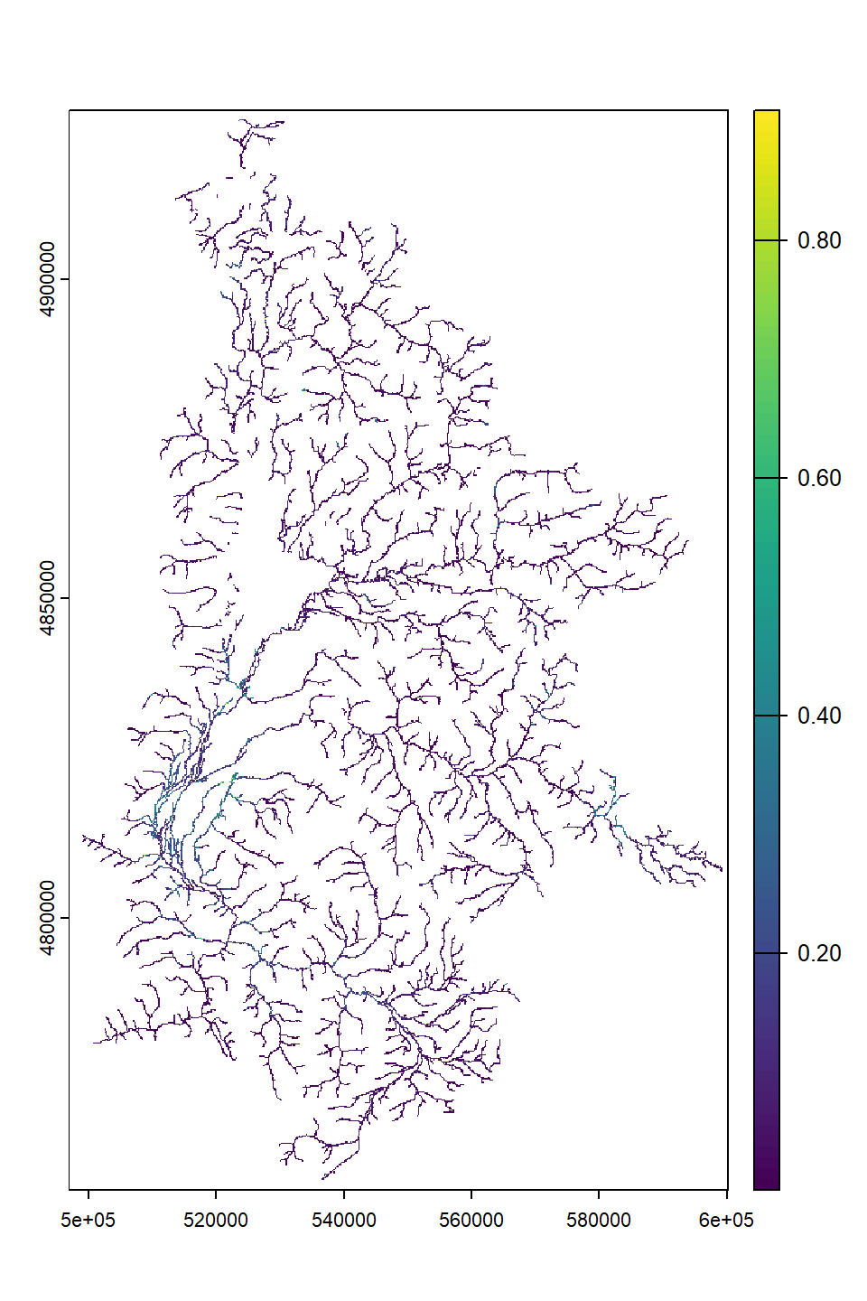

17.2 Box 1

Purpose: Show what high-resolution temporal data (hourly) reveals about network diversity in streamflow response to individual storms (peak flow magnitude and timing and recession rates) and during low flow (diel fluctuations)

17.3 Box 2

The Wedge Model for the West Brook

Purpose: At coarser time scales (summarized by event/baseflow periods), show how streamflow heterogeneity expands and contracts during wet to dry periods.

17.4 Box 3

Purpose: Show what high-resolution spatial data reveals about network diversity in streamflow at a single point in time.

17.5 Box 4

Purpose: Explore the effect of groundwater on relative summer (July-September) water availability.

17.5.1 PASTA approach

Load PASTA daily derived parameters: summarize as July-September site-specific means (across all years)

Code

pasta <- read_csv("C:/Users/jbaldock/OneDrive - DOI/Documents/USGS/EcoDrought/EcoDrought Working/EcoDrought-Analysis/Covariates/pasta_derived_parameters_daily.csv") %>%
  mutate(Month = month(date)) %>%
  rename(CalendarYear = year) %>%
  filter(Month %in% c(7:9)) %>%
  group_by(site_name) %>%
  summarize(meanRatio = mean(meanRatio, na.rm = TRUE),
            phaseLag = mean(phaseLag, na.rm = TRUE),
            amplitudeRatio = mean(amplitudeRatio, na.rm = TRUE))
pasta

# A tibble: 73 × 4
   site_name           meanRatio phaseLag amplitudeRatio
   <chr>                   <dbl>    <dbl>          <dbl>
 1 Avery Brook             0.891     2.31          0.264
 2 BigCreekLower           0.936     2.22          0.376
 3 BigCreekMiddle          0.840     1.29          0.411
 4 BigCreekUpper           0.664     2.31          0.179
 5 Buck Creek              0.699     1.19          0.353
 6 CoalCreekHeadwaters     0.670     2.11          0.209
 7 CoalCreekLower          0.843     2.91          0.503
 8 CoalCreekMiddle         0.692     1.27          0.223
 9 CoalCreekNorth          0.733     2.49          0.246
10 Crandall Creek          0.758     1.76          0.612
# ℹ 63 more rows

Create flow by groundwater plotting function.

Code

mdaystib <- tibble(Month = c(1:12), mdays = c(31,28,31,30,31,30,31,31,30,31,30,31))

gwflowfun <- function (subbas, years, dropsites, months = c(7:9)) {
  dat_clean %>% 
  filter(subbasin == subbas, CalendarYear %in% years, Month %in% months) %>%
  group_by(site_name, subbasin, designation, CalendarYear) %>% #, Month, MonthName) %>%
  summarise(ss = n(),
            logYield = mean(logYield, na.rm = TRUE)) %>%
  ungroup() %>%
  #left_join(mdaystib) %>%
  mutate(pdays = ss/92#,
         #YearMonth = paste(CalendarYear, "_", Month, sep = "")
         ) %>%
  filter(pdays > 0.9,
         !site_name %in% dropsites) %>%
  group_by(CalendarYear) %>%
  mutate(z_logYield = scale(logYield, center = TRUE, scale = TRUE)[,1]) %>%
  ungroup() %>%
  left_join(pasta) %>%
  ggplot(aes(x = amplitudeRatio, y = z_logYield)) +
  geom_abline(intercept = 0, slope = 0, linetype = 2) +
  geom_smooth(method = "lm", color = "black") +
  geom_point(aes(color = site_name)) +
  facet_wrap(~CalendarYear, nrow = 1) +
  #facet_wrap2(~CalendarYear, nrow = 1, ncol = 5, trim_blank = FALSE) +
  #facet_grid(cols = vars(Month), rows = vars(CalendarYear)) + 
  theme_bw() + theme(panel.grid.major = element_blank(), panel.grid.minor = element_blank()) 
}

Plot the relationship between standardized annual summer mean discharge and amplitude ratio from PASTA, where lower amplitude ratio values are indicative of greater groundwater availability. Mean flow for each site is standardized by year to remove interannual variation in climate/regional water availability

Code

gwflowfun(subbas = "West Brook", dropsites = c("West Brook Reservoir", "Mitchell Brook"), years = c(2020:2024))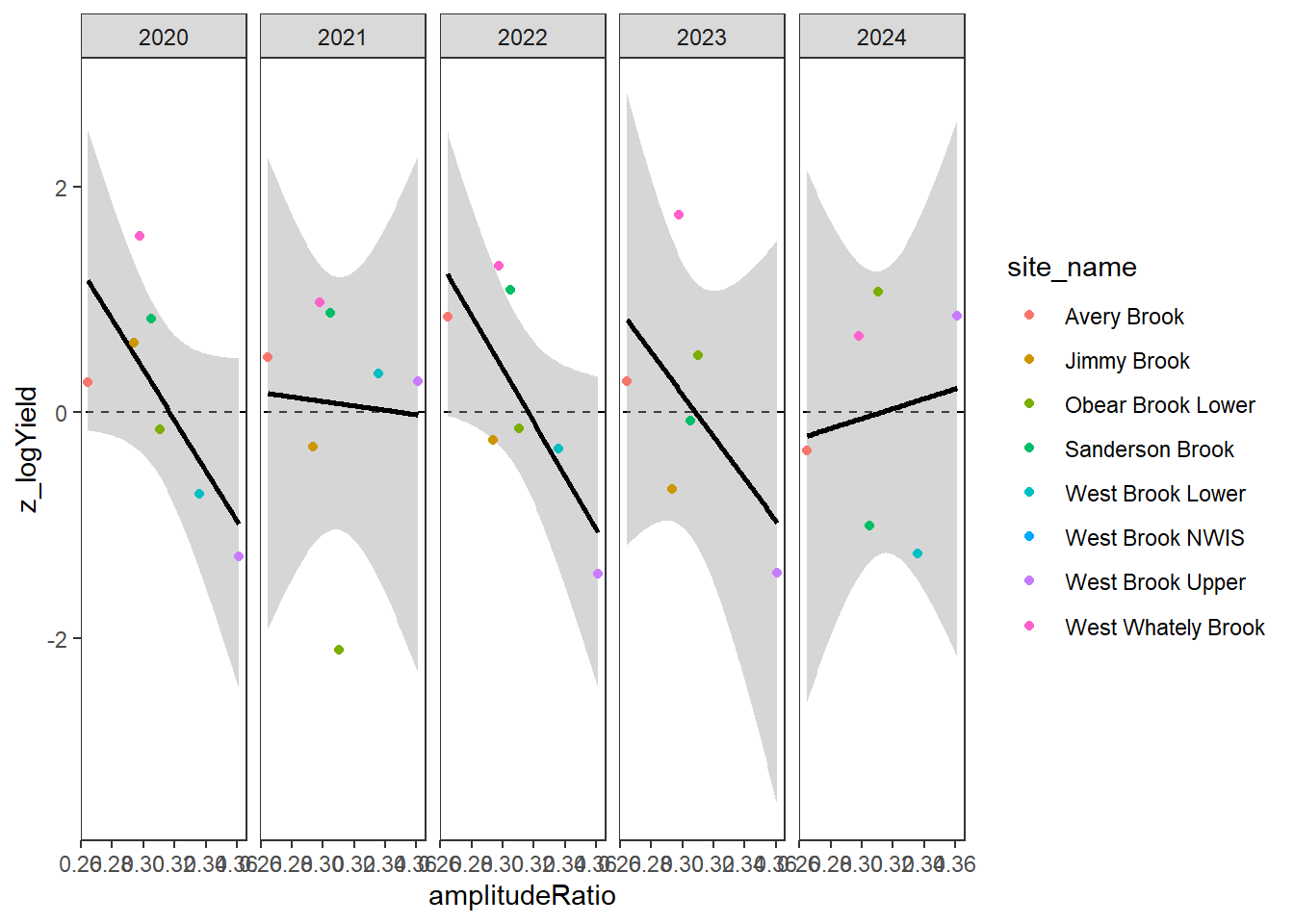

Code

gwflowfun(subbas = "Staunton River", dropsites = NA, years = c(2019:2022))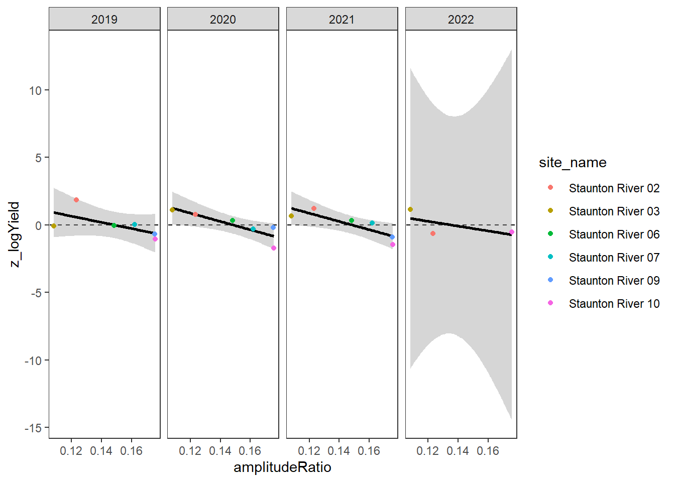

Code

gwflowfun(subbas = "Snake River", dropsites = NA, years = c(2018, 2020:2022), months = c(7:9))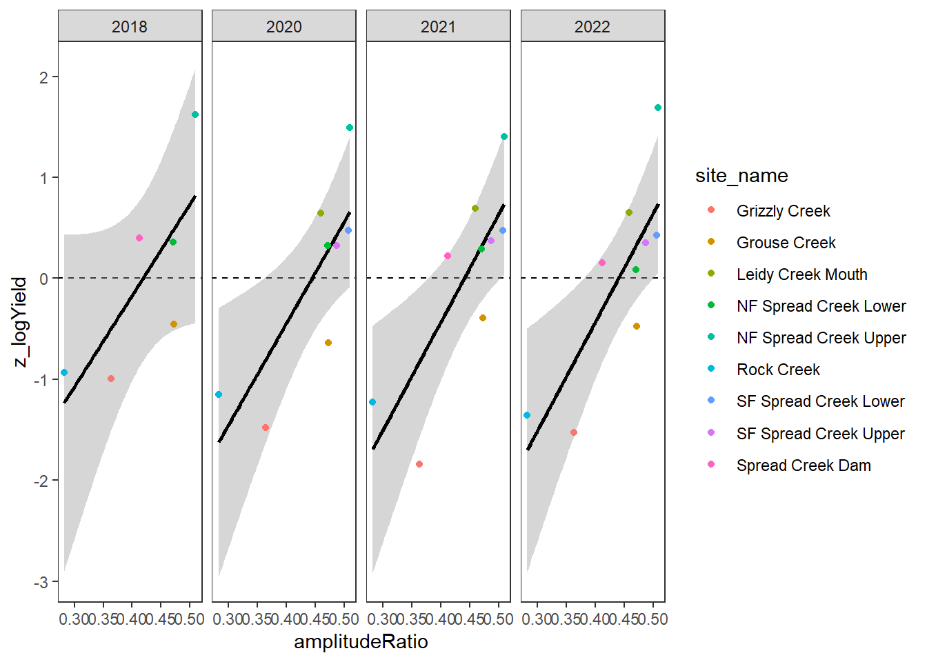

Code

gwflowfun(subbas = "Shields River", dropsites = NA, years = c(2017,2019,2020,2022,2023), months = c(7:9))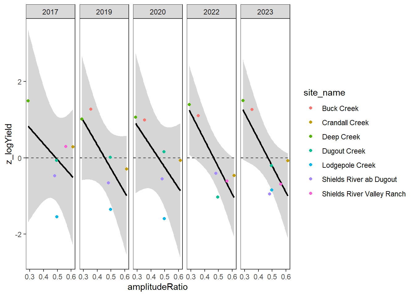

17.5.2 Spring prevalence approach

Extract groundwater metrics from MaxEnt spring prevalence model

Code

# convert to SpatVectors
sites_flow <- vect(siteinfo_sp %>% filter(basin == "Snake River"))
sheds <- vect(sheds)

# transform
sites_flow <- terra::project(sites_flow, crs(springprev))
sheds <- terra::project(sheds, crs(springprev))

# extract average and weighted spring prevalence for each basin
sites <- sheds$site_name
gwlist <- list()
st <- Sys.time()
for (i in 1:length(sites)) {
  spring_mask <- mask(crop(springprev, sheds[sheds$site_name == sites[i],]), sheds[sheds$site_name == sites[i],]) # crop and mask by basin
  dist_rast <- distance(spring_mask, sites_flow[sites_flow$site_name == sites[i],]) %>% mask(spring_mask) # calculate distance between each raster cell and site location
  gwlist[[i]] <- tibble(site_name = sites[i],
                        area_sqmi = sites_flow$area_sqmi[i],
                        springprev_point = terra::extract(springprev, sites_flow[sites_flow$site_name == sites[i],], na.rm = TRUE)[,2],
                        springprev_basinmean = as.numeric(global(spring_mask, "mean", na.rm = T)), # extract(spring_buff, sheds_yoy[sheds_yoy$site == sites[i],], fun = mean, na.rm = TRUE)[,2],
                        springprev_iew01km = as.numeric(global(spring_mask * (1 / exp(dist_rast/1000)), "sum", na.rm = T) / global(1 / exp(dist_rast/1000), "sum", na.rm = T)),
                        springprev_iew05km = as.numeric(global(spring_mask * (1 / exp(dist_rast/5000)), "sum", na.rm = T) / global(1 / exp(dist_rast/5000), "sum", na.rm = T))
                        )
  print(i)
}


|---------|---------|---------|---------|
=========================================
                                          
[1] 1

|---------|---------|---------|---------|
=========================================
                                          
[1] 2

|---------|---------|---------|---------|
=========================================
                                          
[1] 3

|---------|---------|---------|---------|
=========================================
                                          
[1] 4

|---------|---------|---------|---------|
=========================================
                                          
[1] 5

|---------|---------|---------|---------|
=========================================
                                          
[1] 6

|---------|---------|---------|---------|
=========================================
                                          
[1] 7

|---------|---------|---------|---------|
=========================================
                                          
[1] 8

|---------|---------|---------|---------|
=========================================
                                          
[1] 9

|---------|---------|---------|---------|
=========================================
                                          
[1] 10

|---------|---------|---------|---------|
=========================================
                                          
[1] 11

|---------|---------|---------|---------|
=========================================
                                          
[1] 12

|---------|---------|---------|---------|
=========================================
                                          
[1] 13

|---------|---------|---------|---------|
=========================================
                                          
[1] 14

Code

Sys.time() - st

Time difference of 7.001879 secs

Code

gwmetrics_snake <- do.call(rbind, gwlist) # bind as tibble
gwmetrics_snake

# A tibble: 14 × 6
   site_name  area_sqmi springprev_point springprev_basinmean springprev_iew01km
   <chr>          <dbl>            <dbl>                <dbl>              <dbl>
 1 NF Spread…     12.7           0.0441               0.0502             0.0575 
 2 Grouse Cr…      5.15          0.00917              0.0140             0.0104 
 3 Leidy Cre…      5.17          0.00892              0.0320             0.0336 
 4 Leidy Cre…      2.18          0.0305               0.0503             0.0476 
 5 Leidy Cre…      5.16          0.0179               0.0324             0.0369 
 6 NF Spread…     27.9           0.0362               0.0402             0.0223 
 7 Grizzly C…      3.68          0.0379               0.0376             0.0333 
 8 Rock Creek      4.74          0.0175               0.00675            0.00830
 9 SF Spread…     44.3           0.0277               0.0220             0.0119 
10 SF Spread…     35.1           0.00378              0.0245             0.0253 
11 Spread Cr…     97.5           0.0387               0.0286             0.0122 
12 Pacific C…    166.            0.0771               0.0267             0.0442 
13 Leidy Cre…      5.17          0.00634              0.0321             0.0345 
14 SF Spread…     44.2           0.0194               0.0221             0.0119 
# ℹ 1 more variable: springprev_iew05km <dbl>

Plot groundwater index across upper Snake River basin

Code

springprev_cont <- vect("C:/Users/jbaldock/OneDrive - DOI/Documents/USGS/EcoDrought/EcoDrought Working/Data/Snake Groundwater/GroundwaterMetrics_Normalized_PredPoints.shp")
mapview(st_as_sf(springprev_cont), zcol = "springpre3", col.regions = viridis(n = 100, direction = -1))

Plot groundwater index across the Spread Creek sub-watershed (note the change in color scale). This map needs cleaning, but you get the idea

Code

springprev_cont_snake <- mask(crop(springprev_cont, sheds[sheds$site_name == "Spread Creek Dam",]), sheds[sheds$site_name == "Spread Creek Dam",])

mynet <- vect("C:/Users/jbaldock/OneDrive - DOI/Documents/USGS/EcoDrought/EcoDrought Working/EcoDrought-Analysis/Watershed Delineation/Streams/Snake_Streams.shp")
crs(mynet) <- crs(siteinfo_sp)
mynet <- terra::project(mynet, crs(sheds))
mynet <- crop(mynet, sheds[sheds$site_name == "Spread Creek Dam",])

ggplot() +
  geom_sf(data = st_as_sf(sheds[sheds$site_name == "Spread Creek Dam",]), color = "black", fill = "white", linewidth = 0.4) + 
  geom_sf(data = st_as_sf(mynet), color = "white", linewidth = 1, lineend = "round") +
  geom_sf(data = st_as_sf(mynet), color = "royalblue4", linewidth = 0.6, lineend = "round") +
  geom_sf(data = st_as_sf(springprev_cont_snake), aes(colour = springpre3), size = 2) +
  scale_colour_viridis(option = "D", direction = -1, limits = range(springprev_cont_snake$springpre3), na.value = "grey") +
  geom_sf(data = st_as_sf(sites_flow) %>% filter(designation != "big"), shape = 21, fill = "white", size = 2) +
  labs(colour = "Groundwater\nindex") + #annotation_scale() +
  theme_bw() + theme(axis.title.x = element_blank(), axis.title.y = element_blank(), axis.text = element_blank())

Plot relationship between groundwater availability and mean summer log(specific discharge).

Code

dat_summer <- dat_clean %>% 
  filter(basin == "Snake River", Month %in% c(7:9)) %>%
  group_by(site_name, basin, designation, WaterYear) %>% #, Month, MonthName) %>%
  summarise(ndays = n(),
            logYield_mean = mean(logYield, na.rm = TRUE),
            logYield_min = min(logYield, na.rm = TRUE)) %>%
  ungroup() %>%
  mutate(pdays = ndays/92) %>%
  filter(pdays > 0.9) %>%
  left_join(gwmetrics_snake) #%>%
  #left_join(wateravail %>% filter(basin == "Snake River") %>% select(WaterYear, totalyield_sum, totalyield_sum_z))

#summary(lm(logYield_mean ~ springprev_iew05km*totalyield_sum, data = dat_summer))

dat_summer %>%
  #filter(site_name != "Grizzly Creek") %>%
  #filter(WaterYear %in% c(2020:2023)) %>%
  ggplot(aes(x = springprev_iew05km, y = logYield_mean)) +
  geom_smooth(method = "lm", aes(x = springprev_iew05km, y = logYield_mean), se = FALSE, color = "grey50") + 
  geom_point(aes(color = site_name)) + 
  theme_bw() + theme(panel.grid = element_blank()) +
  xlab("Groundwater index") + ylab("Mean summer log(specific discharge)") +
  facet_wrap(~WaterYear)

Code

dat_summer %>%
  filter(WaterYear %in% c(2020:2023)) %>%
  ggplot(aes(x = springprev_iew05km, y = logYield_mean)) +
  geom_smooth(method = "lm", aes(x = springprev_iew05km, y = logYield_mean), se = FALSE, color = "grey50") + 
  geom_point(aes(color = site_name, shape = factor(WaterYear))) + 
  theme_bw() + theme(panel.grid = element_blank()) +
  xlab("Groundwater index") + ylab("Mean summer log(specific discharge)")

With the exception of Grizzly Creek, there is a surprisingly tight relationship between the groundwater index and summer streamflow: higher water availability in reaches with high groundwater availability. Not surprising, but it’s a very nice validation of the MaxEnt approach to estimating groundwater availability and links to summer habitat conditions.

Grizzly is the exception, of course. High groundwater index despite very low flows. I’ve never been there, so I’m wondering what Robert makes of this. One thought I had is that where discharge is measured may be out on an alluvial fan, which may be in a losing reach as water spread outs into more porous material. We built the groundwater model to estimate the prevalence of springs, not where water is lost to the subsurface. So the groundwater index would not reflect these more nuanced dynamics. Alternatively (or additionally), looking at satellite imagery, there is a large beaver complex just upstream of the discharge monitoring site…which may reduce surface flows immediately downstream as shallow sediments are recharged. Scanning satellite imagery, it is pretty clear where springs discharge in the headwaters of Grizzly Creek. So, the MaxEnt model may not necessarily be wrong, but it doesn’t account for other factors which have important effects on streamflow at even finer spatial scales.

This box could have 3 main elements: a photo of a groundwater spring (?), the map of groundwater availability across Spread Creek, and the scatterplots for 2020-2023 (years with good data availability)