Code
siteinfo <- read_csv("C:/Users/jbaldock/OneDrive - DOI/Documents/USGS/EcoDrought/EcoDrought Working/Data/EcoDrought_SiteInformation.csv")
siteinfo_sp <- st_as_sf(siteinfo, coords = c("long", "lat"), crs = 4326)Purpose: Quantify the suitability of existing modeling techniques for predicting streamflow in headwater systems.
Approach:
Site information
siteinfo <- read_csv("C:/Users/jbaldock/OneDrive - DOI/Documents/USGS/EcoDrought/EcoDrought Working/Data/EcoDrought_SiteInformation.csv")
siteinfo_sp <- st_as_sf(siteinfo, coords = c("long", "lat"), crs = 4326)Little g’s
dat_clean <- read_csv("C:/Users/jbaldock/OneDrive - DOI/Documents/USGS/EcoDrought/EcoDrought Working/EcoDrought-Analysis/Qualitative/LittleG_data_clean.csv")Big G’s
dat_clean_big <- read_csv("C:/Users/jbaldock/OneDrive - DOI/Documents/USGS/EcoDrought/EcoDrought Working/EcoDrought-Analysis/Qualitative/BigG_data_clean.csv")Climate
climdf <- read_csv("C:/Users/jbaldock/OneDrive - DOI/Documents/USGS/EcoDrought/EcoDrought Working/EcoDrought-Analysis/Qualitative/Daymet_climate.csv")
climdf_summ <- read_csv("C:/Users/jbaldock/OneDrive - DOI/Documents/USGS/EcoDrought/EcoDrought Working/EcoDrought-Analysis/Qualitative/Daymet_climate_summary.csv")Water availability
wateravail <- read_csv("C:/Users/jbaldock/OneDrive - DOI/Documents/USGS/EcoDrought/EcoDrought Working/EcoDrought-Analysis/Qualitative/BigG_wateravailability_annual.csv")Order sites: for colors, order sites from downstream to upstream (roughly) and by subbasin (if appropriate)
wborder <- c("West Brook NWIS", "West Brook Lower", "Mitchell Brook", "Jimmy Brook", "Obear Brook Lower", "West Brook Upper", "West Brook Reservoir", "Sanderson Brook", "Avery Brook", "West Whately Brook")
paineorder <- c("Paine Run 10", "Paine Run 08", "Paine Run 07", "Paine Run 06", "Paine Run 02", "Paine Run 01")
stauntorder <- c("Staunton River 10", "Staunton River 09", "Staunton River 07", "Staunton River 06", "Staunton River 03", "Staunton River 02")
flatorder <- c("BigCreekLower", "LangfordCreekLower", "LangfordCreekUpper", "Big Creek NWIS", "BigCreekUpper", "HallowattCreekLower", "NicolaCreek", "WernerCreek", "Hallowat Creek NWIS", "CoalCreekLower", "CycloneCreekLower", "CycloneCreekMiddle", "CycloneCreekUpper", "CoalCreekMiddle", "CoalCreekNorth", "CoalCreekHeadwaters", "McGeeCreekLower", "McGeeCreekTrib", "McGeeCreekUpper")
yellorder <- c("Shields River Valley Ranch", "Deep Creek", "Crandall Creek", "Buck Creek", "Dugout Creek", "Shields River ab Dugout", "Lodgepole Creek", "EF Duck Creek be HF", "EF Duck Creek ab HF", "Henrys Fork")
snakeorder <- c("Spread Creek Dam", "Rock Creek", "NF Spread Creek Lower", "NF Spread Creek Upper", "Grizzly Creek", "SF Spread Creek Lower", "Grouse Creek", "SF Spread Creek Upper", "Leidy Creek Mouth")
donnerorder <- c("Fish Creek NWIS", "Donner Blitzen ab Fish NWIS", "Donner Blitzen nr Burnt Car NWIS", "Donner Blitzen ab Indian NWIS")Write out point shape files for each state to feed into Stream Stats batch processor
siteinfo_sp_wy <- siteinfo_sp %>% filter(region == "Snake")
st_write(siteinfo_sp_wy, "C:/Users/jbaldock/OneDrive - DOI/Documents/USGS/EcoDrought/EcoDrought Working/EcoDrought-Analysis/CompareModeledQ/points/points_wy.shp")
siteinfo_sp_mt <- siteinfo_sp %>% filter(region %in% c("Flat", "Shields"))
st_write(siteinfo_sp_mt, "C:/Users/jbaldock/OneDrive - DOI/Documents/USGS/EcoDrought/EcoDrought Working/EcoDrought-Analysis/CompareModeledQ/points/points_mt.shp")
siteinfo_sp_ma <- siteinfo_sp %>% filter(region == "Mass")
st_write(siteinfo_sp_ma, "C:/Users/jbaldock/OneDrive - DOI/Documents/USGS/EcoDrought/EcoDrought Working/EcoDrought-Analysis/CompareModeledQ/points/points_ma.shp")
siteinfo_sp_va <- siteinfo_sp %>% filter(region %in% c("Shen"))
st_write(siteinfo_sp_va, "C:/Users/jbaldock/OneDrive - DOI/Documents/USGS/EcoDrought/EcoDrought Working/EcoDrought-Analysis/CompareModeledQ/points/points_va.shp")
siteinfo_sp_or <- siteinfo_sp %>% filter(region %in% c("Oreg"))
st_write(siteinfo_sp_or, "C:/Users/jbaldock/OneDrive - DOI/Documents/USGS/EcoDrought/EcoDrought Working/EcoDrought-Analysis/CompareModeledQ/points/points_or.shp")List geodatabase layer names
st_layers(dsn = "C:/Users/jbaldock/OneDrive - DOI/Documents/USGS/EcoDrought/EcoDrought Working/EcoDrought-Analysis/CompareModeledQ/StreamStats/points_mt7617/points_mt7617.gdb")Driver: OpenFileGDB
Available layers:
layer_name geometry_type features fields crs_name
1 GlobalWatershedPoint Point 39 8 WGS 84
2 GlobalWatershed Multi Polygon 39 28 WGS 84
3 CHARACTERISTICS NA 1921 11 <NA>
4 FLOWSTATS NA 6763 16 <NA>Read watershed boundaries
sheds_montana <- st_read("C:/Users/jbaldock/OneDrive - DOI/Documents/USGS/EcoDrought/EcoDrought Working/EcoDrought-Analysis/CompareModeledQ/StreamStats/points_mt7617/points_mt7617.gdb", layer = "GlobalWatershed")Reading layer `GlobalWatershed' from data source
`C:\Users\jbaldock\OneDrive - DOI\Documents\USGS\EcoDrought\EcoDrought Working\EcoDrought-Analysis\CompareModeledQ\StreamStats\points_mt7617\points_mt7617.gdb'
using driver `OpenFileGDB'
Simple feature collection with 39 features and 28 fields
Geometry type: MULTIPOLYGON
Dimension: XY
Bounding box: xmin: -114.8904 ymin: 43.9457 xmax: -109.7226 ymax: 49.46148
Geodetic CRS: WGS 84sheds_massach <- st_read("C:/Users/jbaldock/OneDrive - DOI/Documents/USGS/EcoDrought/EcoDrought Working/EcoDrought-Analysis/CompareModeledQ/StreamStats/points_ma7625/points_ma7625.gdb", layer = "GlobalWatershed")Reading layer `GlobalWatershed' from data source
`C:\Users\jbaldock\OneDrive - DOI\Documents\USGS\EcoDrought\EcoDrought Working\EcoDrought-Analysis\CompareModeledQ\StreamStats\points_ma7625\points_ma7625.gdb'
using driver `OpenFileGDB'
Simple feature collection with 13 features and 25 fields
Geometry type: MULTIPOLYGON
Dimension: XY
Bounding box: xmin: -72.82306 ymin: 42.4123 xmax: -72.62871 ymax: 42.54973
Geodetic CRS: WGS 84sheds_oregon <- st_read("C:/Users/jbaldock/OneDrive - DOI/Documents/USGS/EcoDrought/EcoDrought Working/EcoDrought-Analysis/CompareModeledQ/StreamStats/points_or7626/points_or7626.gdb", layer = "GlobalWatershed")Reading layer `GlobalWatershed' from data source
`C:\Users\jbaldock\OneDrive - DOI\Documents\USGS\EcoDrought\EcoDrought Working\EcoDrought-Analysis\CompareModeledQ\StreamStats\points_or7626\points_or7626.gdb'
using driver `OpenFileGDB'
Simple feature collection with 7 features and 41 fields
Geometry type: MULTIPOLYGON
Dimension: XY
Bounding box: xmin: -118.9295 ymin: 42.48917 xmax: -118.561 ymax: 42.79204
Geodetic CRS: WGS 84sheds_virginia <- st_read("C:/Users/jbaldock/OneDrive - DOI/Documents/USGS/EcoDrought/EcoDrought Working/EcoDrought-Analysis/CompareModeledQ/StreamStats/points_va7627/points_va7627.gdb", layer = "GlobalWatershed")Reading layer `GlobalWatershed' from data source
`C:\Users\jbaldock\OneDrive - DOI\Documents\USGS\EcoDrought\EcoDrought Working\EcoDrought-Analysis\CompareModeledQ\StreamStats\points_va7627\points_va7627.gdb'
using driver `OpenFileGDB'
Simple feature collection with 32 features and 20 fields
Geometry type: MULTIPOLYGON
Dimension: XY
Bounding box: xmin: -79.24034 ymin: 37.88165 xmax: -78.02949 ymax: 38.7622
Geodetic CRS: WGS 84sheds_wyoming <- st_read("C:/Users/jbaldock/OneDrive - DOI/Documents/USGS/EcoDrought/EcoDrought Working/EcoDrought-Analysis/CompareModeledQ/StreamStats/points_wy7628/points_wy7628.gdb", layer = "GlobalWatershed")Reading layer `GlobalWatershed' from data source
`C:\Users\jbaldock\OneDrive - DOI\Documents\USGS\EcoDrought\EcoDrought Working\EcoDrought-Analysis\CompareModeledQ\StreamStats\points_wy7628\points_wy7628.gdb'
using driver `OpenFileGDB'
Simple feature collection with 14 features and 17 fields
Geometry type: MULTIPOLYGON
Dimension: XY
Bounding box: xmin: -110.5241 ymin: 43.64373 xmax: -110.1598 ymax: 43.87029
Geodetic CRS: WGS 84sheds <- bind_rows(sheds_massach, sheds_montana, sheds_oregon, sheds_virginia, sheds_wyoming)
mapview(sheds) Find sites that were delineated incorrectly
options(scipen=999)
badsites <- tibble(sheds) %>% select(Name, Shape_Area, DRNAREA, ELEV) %>% rename(site_id = Name) %>% left_join(siteinfo %>% select(site_id, site_name, area_sqmi, elev_ft)) %>% select(site_id, site_name, DRNAREA, area_sqmi) %>% mutate(percerror = (DRNAREA - area_sqmi) / area_sqmi) %>% filter(percerror >= 0.15 | percerror <= -0.15)
badsites# A tibble: 15 × 5
site_id site_name DRNAREA area_sqmi percerror
<chr> <chr> <dbl> <dbl> <dbl>
1 WW West Whately Brook 0.0399 0.493 -0.919
2 WL West Brook Lower 0.086 8.51 -0.990
3 JB Jimmy Brook 7.87 0.974 7.08
4 SH08 Shields River ab Dugout 11.1 8.68 0.279
5 SH06 Lodgepole Creek 2.2 1.36 0.619
6 SH05 Dugout Creek 11.1 2.39 3.64
7 BIG_002 LangfordCreekLower 0.1 3.99 -0.975
8 RAP Rapidan River NWIS 0.0000386 115 -1.000
9 PI_09FL Piney River 09 0.36 4.28 -0.916
10 LEI Leidy Creek Mouth NWIS 0.000811 5.17 -1.000
11 PCM Pacific Creek at Moran NWIS 0.34 166. -0.998
12 SP10 SF Spread Creek Upper 0.000348 35.1 -1.000
13 SP09 SF Spread Creek Lower 72 44.3 0.627
14 SP08 Rock Creek 0.0000772 4.74 -1.000
15 SP03 Leidy Creek Lower 0.00112 5.17 -1.000Stream stats site information
streamstats_info <- tibble(sheds) %>% select(Name, DRNAREA) %>% rename(site_id = Name) %>% left_join(siteinfo %>% select(site_id, site_name))
# streamstats_infoRead flow statistics from geodatabases
montana <- st_read("C:/Users/jbaldock/OneDrive - DOI/Documents/USGS/EcoDrought/EcoDrought Working/EcoDrought-Analysis/CompareModeledQ/StreamStats/points_mt7617/points_mt7617.gdb", layer = "FLOWSTATS")Reading layer `FLOWSTATS' from data source
`C:\Users\jbaldock\OneDrive - DOI\Documents\USGS\EcoDrought\EcoDrought Working\EcoDrought-Analysis\CompareModeledQ\StreamStats\points_mt7617\points_mt7617.gdb'
using driver `OpenFileGDB'massach <- st_read("C:/Users/jbaldock/OneDrive - DOI/Documents/USGS/EcoDrought/EcoDrought Working/EcoDrought-Analysis/CompareModeledQ/StreamStats/points_ma7625/points_ma7625.gdb", layer = "FLOWSTATS")Reading layer `FLOWSTATS' from data source
`C:\Users\jbaldock\OneDrive - DOI\Documents\USGS\EcoDrought\EcoDrought Working\EcoDrought-Analysis\CompareModeledQ\StreamStats\points_ma7625\points_ma7625.gdb'
using driver `OpenFileGDB'oregon <- st_read("C:/Users/jbaldock/OneDrive - DOI/Documents/USGS/EcoDrought/EcoDrought Working/EcoDrought-Analysis/CompareModeledQ/StreamStats/points_or7626/points_or7626.gdb", layer = "FLOWSTATS")Reading layer `FLOWSTATS' from data source
`C:\Users\jbaldock\OneDrive - DOI\Documents\USGS\EcoDrought\EcoDrought Working\EcoDrought-Analysis\CompareModeledQ\StreamStats\points_or7626\points_or7626.gdb'
using driver `OpenFileGDB'virginia <- st_read("C:/Users/jbaldock/OneDrive - DOI/Documents/USGS/EcoDrought/EcoDrought Working/EcoDrought-Analysis/CompareModeledQ/StreamStats/points_va7627/points_va7627.gdb", layer = "FLOWSTATS")Reading layer `FLOWSTATS' from data source
`C:\Users\jbaldock\OneDrive - DOI\Documents\USGS\EcoDrought\EcoDrought Working\EcoDrought-Analysis\CompareModeledQ\StreamStats\points_va7627\points_va7627.gdb'
using driver `OpenFileGDB'wyoming <- st_read("C:/Users/jbaldock/OneDrive - DOI/Documents/USGS/EcoDrought/EcoDrought Working/EcoDrought-Analysis/CompareModeledQ/StreamStats/points_wy7628/points_wy7628.gdb", layer = "FLOWSTATS")Reading layer `FLOWSTATS' from data source
`C:\Users\jbaldock\OneDrive - DOI\Documents\USGS\EcoDrought\EcoDrought Working\EcoDrought-Analysis\CompareModeledQ\StreamStats\points_wy7628\points_wy7628.gdb'
using driver `OpenFileGDB'streamstats <- bind_rows(montana, massach, oregon, virginia, wyoming) %>% filter(!Name %in% c(badsites$site_id)) %>% rename(site_id = Name) %>% left_join(siteinfo %>% select(site_id, site_name)) %>% left_join(streamstats_info)
head(streamstats) site_id RegionID RegionName AreaPercent AreaSqMi
1 NFF GC1906 Crippen_Bue_Region_13 61 947.3549
2 NFF GC1828 USA_Bieger_2015 60 937.1283
3 NFF GC1828 USA_Bieger_2015 60 937.1283
4 NFF GC1828 USA_Bieger_2015 60 937.1283
5 NFF GC1818 Northern_Rocky_Mountains_P_Bieger_2015 60 937.1283
6 NFF GC1818 Northern_Rocky_Mountains_P_Bieger_2015 60 937.1283
StatLabel StatName Value
1 PKMAX_CB_R Maximum Flood Crippen Bue Regional 246000.00
2 XABNKF_U_B Bieger_USA_channel_cross_sectional_area 905.00
3 DBANKF_U_B Bieger_USA_channel_depth 5.77
4 WBANKF_U_B Bieger_USA_channel_width 165.00
5 XABNKF_P_B Bieger_P_channel_cross_sectional_area 852.00
6 DBANKF_P_B Bieger_P_channel_depth 5.53
Units Years PIl PIu SE SEp PC CitationID
1 cubic feet per second NA NA NA NA NA NA 186
2 square feet 0 NA NA NA NA NA 160
3 feet 0 NA NA NA NA NA 160
4 feet 0 NA NA NA NA NA 160
5 square feet 0 NA NA NA NA NA 160
6 feet 0 NA NA NA NA NA 160
site_name DRNAREA
1 North Fork Flathead River NWIS 1556.2
2 North Fork Flathead River NWIS 1556.2
3 North Fork Flathead River NWIS 1556.2
4 North Fork Flathead River NWIS 1556.2
5 North Fork Flathead River NWIS 1556.2
6 North Fork Flathead River NWIS 1556.2char_massach <- st_read("C:/Users/jbaldock/OneDrive - DOI/Documents/USGS/EcoDrought/EcoDrought Working/EcoDrought-Analysis/CompareModeledQ/StreamStats/points_ma7625/points_ma7625.gdb", layer = "CHARACTERISTICS")Reading layer `CHARACTERISTICS' from data source
`C:\Users\jbaldock\OneDrive - DOI\Documents\USGS\EcoDrought\EcoDrought Working\EcoDrought-Analysis\CompareModeledQ\StreamStats\points_ma7625\points_ma7625.gdb'
using driver `OpenFileGDB'char_massach Name RegionID RegionName AreaPercent AreaSqMi
1 WBR GC1894 Crippen_Bue_Region_1 100 10.70496118
2 WBR GC828 Perennial_Flow_Probability 100 10.70496118
3 WBR GC828 Perennial_Flow_Probability 100 10.70496118
4 WBR GC828 Perennial_Flow_Probability 100 10.70496118
5 WBR GC828 Perennial_Flow_Probability 100 10.70496118
6 WBR GC1828 USA_Bieger_2015 100 10.70496118
7 WBR GC1807 New_England_P_Bieger_2015 100 10.70496118
8 WBR GC1804 Appalachian_Highlands_D_Bieger_2015 100 10.70496118
9 WBR GC1594 Bankfull_Statewide_SIR2013_5155 100 10.70496118
10 WBR GC1594 Bankfull_Statewide_SIR2013_5155 100 10.70496118
11 WBR GC320 Statewide_Low_Flow_WRIR00_4135 100 10.70496118
12 WBR GC320 Statewide_Low_Flow_WRIR00_4135 100 10.70496118
13 WBR GC320 Statewide_Low_Flow_WRIR00_4135 100 10.70496118
14 WBR GC320 Statewide_Low_Flow_WRIR00_4135 100 10.70496118
15 WBR GC320 Statewide_Low_Flow_WRIR00_4135 100 10.70496118
16 WBR GC320 Statewide_Low_Flow_WRIR00_4135 100 10.70496118
17 WBR GC320 Statewide_Low_Flow_WRIR00_4135 100 10.70496118
18 WBR GC320 Statewide_Low_Flow_WRIR00_4135 100 10.70496118
19 WBR GC320 Statewide_Low_Flow_WRIR00_4135 100 10.70496118
20 WBR GC320 Statewide_Low_Flow_WRIR00_4135 100 10.70496118
21 WBR GC320 Statewide_Low_Flow_WRIR00_4135 100 10.70496118
22 WBR GC320 Statewide_Low_Flow_WRIR00_4135 100 10.70496118
23 WBR GC1741 Peak_Statewide_2016_5156 100 10.70496118
24 WBR GC1741 Peak_Statewide_2016_5156 100 10.70496118
25 WBR GC1741 Peak_Statewide_2016_5156 100 10.70496118
26 AVB GC1894 Crippen_Bue_Region_1 100 3.03310618
27 AVB GC828 Perennial_Flow_Probability 100 3.03310618
28 AVB GC828 Perennial_Flow_Probability 100 3.03310618
29 AVB GC828 Perennial_Flow_Probability 100 3.03310618
30 AVB GC828 Perennial_Flow_Probability 100 3.03310618
31 AVB GC1828 USA_Bieger_2015 100 3.03310618
32 AVB GC1807 New_England_P_Bieger_2015 100 3.03310618
33 AVB GC1804 Appalachian_Highlands_D_Bieger_2015 100 3.03310618
34 AVB GC1594 Bankfull_Statewide_SIR2013_5155 100 3.03310618
35 AVB GC1594 Bankfull_Statewide_SIR2013_5155 100 3.03310618
36 AVB GC320 Statewide_Low_Flow_WRIR00_4135 100 3.03310618
37 AVB GC320 Statewide_Low_Flow_WRIR00_4135 100 3.03310618
38 AVB GC320 Statewide_Low_Flow_WRIR00_4135 100 3.03310618
39 AVB GC320 Statewide_Low_Flow_WRIR00_4135 100 3.03310618
40 AVB GC320 Statewide_Low_Flow_WRIR00_4135 100 3.03310618
41 AVB GC320 Statewide_Low_Flow_WRIR00_4135 100 3.03310618
42 AVB GC320 Statewide_Low_Flow_WRIR00_4135 100 3.03310618
43 AVB GC320 Statewide_Low_Flow_WRIR00_4135 100 3.03310618
44 AVB GC320 Statewide_Low_Flow_WRIR00_4135 100 3.03310618
45 AVB GC320 Statewide_Low_Flow_WRIR00_4135 100 3.03310618
46 AVB GC320 Statewide_Low_Flow_WRIR00_4135 100 3.03310618
47 AVB GC320 Statewide_Low_Flow_WRIR00_4135 100 3.03310618
48 AVB GC1741 Peak_Statewide_2016_5156 100 3.03310618
49 AVB GC1741 Peak_Statewide_2016_5156 100 3.03310618
50 AVB GC1741 Peak_Statewide_2016_5156 100 3.03310618
51 SRC GC1894 Crippen_Bue_Region_1 100 24.06326178
52 SRC GC828 Perennial_Flow_Probability 100 24.06326178
53 SRC GC828 Perennial_Flow_Probability 100 24.06326178
54 SRC GC828 Perennial_Flow_Probability 100 24.06326178
55 SRC GC828 Perennial_Flow_Probability 100 24.06326178
56 SRC GC1828 USA_Bieger_2015 100 24.06326178
57 SRC GC1807 New_England_P_Bieger_2015 100 24.06326178
58 SRC GC1804 Appalachian_Highlands_D_Bieger_2015 100 24.06326178
59 SRC GC1594 Bankfull_Statewide_SIR2013_5155 100 24.06326178
60 SRC GC1594 Bankfull_Statewide_SIR2013_5155 100 24.06326178
61 SRC GC320 Statewide_Low_Flow_WRIR00_4135 100 24.06326178
62 SRC GC320 Statewide_Low_Flow_WRIR00_4135 100 24.06326178
63 SRC GC320 Statewide_Low_Flow_WRIR00_4135 100 24.06326178
64 SRC GC320 Statewide_Low_Flow_WRIR00_4135 100 24.06326178
65 SRC GC320 Statewide_Low_Flow_WRIR00_4135 100 24.06326178
66 SRC GC320 Statewide_Low_Flow_WRIR00_4135 100 24.06326178
67 SRC GC320 Statewide_Low_Flow_WRIR00_4135 100 24.06326178
68 SRC GC320 Statewide_Low_Flow_WRIR00_4135 100 24.06326178
69 SRC GC320 Statewide_Low_Flow_WRIR00_4135 100 24.06326178
70 SRC GC320 Statewide_Low_Flow_WRIR00_4135 100 24.06326178
71 SRC GC320 Statewide_Low_Flow_WRIR00_4135 100 24.06326178
72 SRC GC320 Statewide_Low_Flow_WRIR00_4135 100 24.06326178
73 SRC GC1741 Peak_Statewide_2016_5156 100 24.06326178
74 SRC GC1741 Peak_Statewide_2016_5156 100 24.06326178
75 SRC GC1741 Peak_Statewide_2016_5156 100 24.06326178
76 WM GC1894 Crippen_Bue_Region_1 100 10.70113854
77 WM GC828 Perennial_Flow_Probability 100 10.70113854
78 WM GC828 Perennial_Flow_Probability 100 10.70113854
79 WM GC828 Perennial_Flow_Probability 100 10.70113854
80 WM GC828 Perennial_Flow_Probability 100 10.70113854
81 WM GC1828 USA_Bieger_2015 100 10.70113854
82 WM GC1807 New_England_P_Bieger_2015 100 10.70113854
83 WM GC1804 Appalachian_Highlands_D_Bieger_2015 100 10.70113854
84 WM GC1594 Bankfull_Statewide_SIR2013_5155 100 10.70113854
85 WM GC1594 Bankfull_Statewide_SIR2013_5155 100 10.70113854
86 WM GC320 Statewide_Low_Flow_WRIR00_4135 100 10.70113854
87 WM GC320 Statewide_Low_Flow_WRIR00_4135 100 10.70113854
88 WM GC320 Statewide_Low_Flow_WRIR00_4135 100 10.70113854
89 WM GC320 Statewide_Low_Flow_WRIR00_4135 100 10.70113854
90 WM GC320 Statewide_Low_Flow_WRIR00_4135 100 10.70113854
91 WM GC320 Statewide_Low_Flow_WRIR00_4135 100 10.70113854
92 WM GC320 Statewide_Low_Flow_WRIR00_4135 100 10.70113854
93 WM GC320 Statewide_Low_Flow_WRIR00_4135 100 10.70113854
94 WM GC320 Statewide_Low_Flow_WRIR00_4135 100 10.70113854
95 WM GC320 Statewide_Low_Flow_WRIR00_4135 100 10.70113854
96 WM GC320 Statewide_Low_Flow_WRIR00_4135 100 10.70113854
97 WM GC320 Statewide_Low_Flow_WRIR00_4135 100 10.70113854
98 WM GC1741 Peak_Statewide_2016_5156 100 10.70113854
99 WM GC1741 Peak_Statewide_2016_5156 100 10.70113854
100 WM GC1741 Peak_Statewide_2016_5156 100 10.70113854
101 WW GC1894 Crippen_Bue_Region_1 100 0.03992504
102 WW GC828 Perennial_Flow_Probability 100 0.03992504
103 WW GC828 Perennial_Flow_Probability 100 0.03992504
104 WW GC828 Perennial_Flow_Probability 100 0.03992504
105 WW GC828 Perennial_Flow_Probability 100 0.03992504
106 WW GC1828 USA_Bieger_2015 100 0.03992504
107 WW GC1807 New_England_P_Bieger_2015 100 0.03992504
108 WW GC1804 Appalachian_Highlands_D_Bieger_2015 100 0.03992504
109 WW GC1594 Bankfull_Statewide_SIR2013_5155 100 0.03992504
110 WW GC1594 Bankfull_Statewide_SIR2013_5155 100 0.03992504
111 WW GC320 Statewide_Low_Flow_WRIR00_4135 100 0.03992504
112 WW GC320 Statewide_Low_Flow_WRIR00_4135 100 0.03992504
113 WW GC320 Statewide_Low_Flow_WRIR00_4135 100 0.03992504
114 WW GC320 Statewide_Low_Flow_WRIR00_4135 100 0.03992504
115 WW GC320 Statewide_Low_Flow_WRIR00_4135 100 0.03992504
116 WW GC320 Statewide_Low_Flow_WRIR00_4135 100 0.03992504
117 WW GC320 Statewide_Low_Flow_WRIR00_4135 100 0.03992504
118 WW GC320 Statewide_Low_Flow_WRIR00_4135 100 0.03992504
119 WW GC320 Statewide_Low_Flow_WRIR00_4135 100 0.03992504
120 WW GC320 Statewide_Low_Flow_WRIR00_4135 100 0.03992504
121 WW GC320 Statewide_Low_Flow_WRIR00_4135 100 0.03992504
122 WW GC320 Statewide_Low_Flow_WRIR00_4135 100 0.03992504
123 WW GC1741 Peak_Statewide_2016_5156 100 0.03992504
124 WW GC1741 Peak_Statewide_2016_5156 100 0.03992504
125 WW GC1741 Peak_Statewide_2016_5156 100 0.03992504
126 WR GC1894 Crippen_Bue_Region_1 100 6.18252206
127 WR GC828 Perennial_Flow_Probability 100 6.18252206
128 WR GC828 Perennial_Flow_Probability 100 6.18252206
129 WR GC828 Perennial_Flow_Probability 100 6.18252206
130 WR GC828 Perennial_Flow_Probability 100 6.18252206
131 WR GC1828 USA_Bieger_2015 100 6.18252206
132 WR GC1807 New_England_P_Bieger_2015 100 6.18252206
133 WR GC1804 Appalachian_Highlands_D_Bieger_2015 100 6.18252206
134 WR GC1594 Bankfull_Statewide_SIR2013_5155 100 6.18252206
135 WR GC1594 Bankfull_Statewide_SIR2013_5155 100 6.18252206
136 WR GC320 Statewide_Low_Flow_WRIR00_4135 100 6.18252206
137 WR GC320 Statewide_Low_Flow_WRIR00_4135 100 6.18252206
138 WR GC320 Statewide_Low_Flow_WRIR00_4135 100 6.18252206
139 WR GC320 Statewide_Low_Flow_WRIR00_4135 100 6.18252206
140 WR GC320 Statewide_Low_Flow_WRIR00_4135 100 6.18252206
141 WR GC320 Statewide_Low_Flow_WRIR00_4135 100 6.18252206
142 WR GC320 Statewide_Low_Flow_WRIR00_4135 100 6.18252206
143 WR GC320 Statewide_Low_Flow_WRIR00_4135 100 6.18252206
144 WR GC320 Statewide_Low_Flow_WRIR00_4135 100 6.18252206
145 WR GC320 Statewide_Low_Flow_WRIR00_4135 100 6.18252206
146 WR GC320 Statewide_Low_Flow_WRIR00_4135 100 6.18252206
147 WR GC320 Statewide_Low_Flow_WRIR00_4135 100 6.18252206
148 WR GC1741 Peak_Statewide_2016_5156 100 6.18252206
149 WR GC1741 Peak_Statewide_2016_5156 100 6.18252206
150 WR GC1741 Peak_Statewide_2016_5156 100 6.18252206
151 WU GC1894 Crippen_Bue_Region_1 100 6.30944092
152 WU GC828 Perennial_Flow_Probability 100 6.30944092
153 WU GC828 Perennial_Flow_Probability 100 6.30944092
154 WU GC828 Perennial_Flow_Probability 100 6.30944092
155 WU GC828 Perennial_Flow_Probability 100 6.30944092
156 WU GC1828 USA_Bieger_2015 100 6.30944092
157 WU GC1807 New_England_P_Bieger_2015 100 6.30944092
158 WU GC1804 Appalachian_Highlands_D_Bieger_2015 100 6.30944092
159 WU GC1594 Bankfull_Statewide_SIR2013_5155 100 6.30944092
160 WU GC1594 Bankfull_Statewide_SIR2013_5155 100 6.30944092
161 WU GC320 Statewide_Low_Flow_WRIR00_4135 100 6.30944092
162 WU GC320 Statewide_Low_Flow_WRIR00_4135 100 6.30944092
163 WU GC320 Statewide_Low_Flow_WRIR00_4135 100 6.30944092
164 WU GC320 Statewide_Low_Flow_WRIR00_4135 100 6.30944092
165 WU GC320 Statewide_Low_Flow_WRIR00_4135 100 6.30944092
166 WU GC320 Statewide_Low_Flow_WRIR00_4135 100 6.30944092
167 WU GC320 Statewide_Low_Flow_WRIR00_4135 100 6.30944092
168 WU GC320 Statewide_Low_Flow_WRIR00_4135 100 6.30944092
169 WU GC320 Statewide_Low_Flow_WRIR00_4135 100 6.30944092
170 WU GC320 Statewide_Low_Flow_WRIR00_4135 100 6.30944092
171 WU GC320 Statewide_Low_Flow_WRIR00_4135 100 6.30944092
172 WU GC320 Statewide_Low_Flow_WRIR00_4135 100 6.30944092
173 WU GC1741 Peak_Statewide_2016_5156 100 6.30944092
174 WU GC1741 Peak_Statewide_2016_5156 100 6.30944092
175 WU GC1741 Peak_Statewide_2016_5156 100 6.30944092
176 WL GC1894 Crippen_Bue_Region_1 100 0.08595118
177 WL GC828 Perennial_Flow_Probability 100 0.08595118
178 WL GC828 Perennial_Flow_Probability 100 0.08595118
179 WL GC828 Perennial_Flow_Probability 100 0.08595118
180 WL GC828 Perennial_Flow_Probability 100 0.08595118
181 WL GC1828 USA_Bieger_2015 100 0.08595118
182 WL GC1807 New_England_P_Bieger_2015 100 0.08595118
183 WL GC1804 Appalachian_Highlands_D_Bieger_2015 100 0.08595118
184 WL GC1594 Bankfull_Statewide_SIR2013_5155 100 0.08595118
185 WL GC1594 Bankfull_Statewide_SIR2013_5155 100 0.08595118
186 WL GC320 Statewide_Low_Flow_WRIR00_4135 100 0.08595118
187 WL GC320 Statewide_Low_Flow_WRIR00_4135 100 0.08595118
188 WL GC320 Statewide_Low_Flow_WRIR00_4135 100 0.08595118
189 WL GC320 Statewide_Low_Flow_WRIR00_4135 100 0.08595118
190 WL GC320 Statewide_Low_Flow_WRIR00_4135 100 0.08595118
191 WL GC320 Statewide_Low_Flow_WRIR00_4135 100 0.08595118
192 WL GC320 Statewide_Low_Flow_WRIR00_4135 100 0.08595118
193 WL GC320 Statewide_Low_Flow_WRIR00_4135 100 0.08595118
194 WL GC320 Statewide_Low_Flow_WRIR00_4135 100 0.08595118
195 WL GC320 Statewide_Low_Flow_WRIR00_4135 100 0.08595118
196 WL GC320 Statewide_Low_Flow_WRIR00_4135 100 0.08595118
197 WL GC320 Statewide_Low_Flow_WRIR00_4135 100 0.08595118
198 WL GC1741 Peak_Statewide_2016_5156 100 0.08595118
199 WL GC1741 Peak_Statewide_2016_5156 100 0.08595118
200 WL GC1741 Peak_Statewide_2016_5156 100 0.08595118
201 SD GC1894 Crippen_Bue_Region_1 100 1.65002328
202 SD GC828 Perennial_Flow_Probability 100 1.65002328
203 SD GC828 Perennial_Flow_Probability 100 1.65002328
204 SD GC828 Perennial_Flow_Probability 100 1.65002328
205 SD GC828 Perennial_Flow_Probability 100 1.65002328
206 SD GC1828 USA_Bieger_2015 100 1.65002328
207 SD GC1807 New_England_P_Bieger_2015 100 1.65002328
208 SD GC1804 Appalachian_Highlands_D_Bieger_2015 100 1.65002328
209 SD GC1594 Bankfull_Statewide_SIR2013_5155 100 1.65002328
210 SD GC1594 Bankfull_Statewide_SIR2013_5155 100 1.65002328
211 SD GC320 Statewide_Low_Flow_WRIR00_4135 100 1.65002328
212 SD GC320 Statewide_Low_Flow_WRIR00_4135 100 1.65002328
213 SD GC320 Statewide_Low_Flow_WRIR00_4135 100 1.65002328
214 SD GC320 Statewide_Low_Flow_WRIR00_4135 100 1.65002328
215 SD GC320 Statewide_Low_Flow_WRIR00_4135 100 1.65002328
216 SD GC320 Statewide_Low_Flow_WRIR00_4135 100 1.65002328
217 SD GC320 Statewide_Low_Flow_WRIR00_4135 100 1.65002328
218 SD GC320 Statewide_Low_Flow_WRIR00_4135 100 1.65002328
219 SD GC320 Statewide_Low_Flow_WRIR00_4135 100 1.65002328
220 SD GC320 Statewide_Low_Flow_WRIR00_4135 100 1.65002328
221 SD GC320 Statewide_Low_Flow_WRIR00_4135 100 1.65002328
222 SD GC320 Statewide_Low_Flow_WRIR00_4135 100 1.65002328
223 SD GC1741 Peak_Statewide_2016_5156 100 1.65002328
224 SD GC1741 Peak_Statewide_2016_5156 100 1.65002328
225 SD GC1741 Peak_Statewide_2016_5156 100 1.65002328
226 OL GC1894 Crippen_Bue_Region_1 100 0.52505181
227 OL GC828 Perennial_Flow_Probability 100 0.52505181
228 OL GC828 Perennial_Flow_Probability 100 0.52505181
229 OL GC828 Perennial_Flow_Probability 100 0.52505181
230 OL GC828 Perennial_Flow_Probability 100 0.52505181
231 OL GC1828 USA_Bieger_2015 100 0.52505181
232 OL GC1807 New_England_P_Bieger_2015 100 0.52505181
233 OL GC1804 Appalachian_Highlands_D_Bieger_2015 100 0.52505181
234 OL GC1594 Bankfull_Statewide_SIR2013_5155 100 0.52505181
235 OL GC1594 Bankfull_Statewide_SIR2013_5155 100 0.52505181
236 OL GC320 Statewide_Low_Flow_WRIR00_4135 100 0.52505181
237 OL GC320 Statewide_Low_Flow_WRIR00_4135 100 0.52505181
238 OL GC320 Statewide_Low_Flow_WRIR00_4135 100 0.52505181
239 OL GC320 Statewide_Low_Flow_WRIR00_4135 100 0.52505181
240 OL GC320 Statewide_Low_Flow_WRIR00_4135 100 0.52505181
241 OL GC320 Statewide_Low_Flow_WRIR00_4135 100 0.52505181
242 OL GC320 Statewide_Low_Flow_WRIR00_4135 100 0.52505181
243 OL GC320 Statewide_Low_Flow_WRIR00_4135 100 0.52505181
244 OL GC320 Statewide_Low_Flow_WRIR00_4135 100 0.52505181
245 OL GC320 Statewide_Low_Flow_WRIR00_4135 100 0.52505181
246 OL GC320 Statewide_Low_Flow_WRIR00_4135 100 0.52505181
247 OL GC320 Statewide_Low_Flow_WRIR00_4135 100 0.52505181
248 OL GC1741 Peak_Statewide_2016_5156 100 0.52505181
249 OL GC1741 Peak_Statewide_2016_5156 100 0.52505181
250 OL GC1741 Peak_Statewide_2016_5156 100 0.52505181
251 MB GC1894 Crippen_Bue_Region_1 100 0.38423149
252 MB GC828 Perennial_Flow_Probability 100 0.38423149
253 MB GC828 Perennial_Flow_Probability 100 0.38423149
254 MB GC828 Perennial_Flow_Probability 100 0.38423149
255 MB GC828 Perennial_Flow_Probability 100 0.38423149
256 MB GC1828 USA_Bieger_2015 100 0.38423149
257 MB GC1807 New_England_P_Bieger_2015 100 0.38423149
258 MB GC1804 Appalachian_Highlands_D_Bieger_2015 100 0.38423149
259 MB GC1594 Bankfull_Statewide_SIR2013_5155 100 0.38423149
260 MB GC1594 Bankfull_Statewide_SIR2013_5155 100 0.38423149
261 MB GC320 Statewide_Low_Flow_WRIR00_4135 100 0.38423149
262 MB GC320 Statewide_Low_Flow_WRIR00_4135 100 0.38423149
263 MB GC320 Statewide_Low_Flow_WRIR00_4135 100 0.38423149
264 MB GC320 Statewide_Low_Flow_WRIR00_4135 100 0.38423149
265 MB GC320 Statewide_Low_Flow_WRIR00_4135 100 0.38423149
266 MB GC320 Statewide_Low_Flow_WRIR00_4135 100 0.38423149
267 MB GC320 Statewide_Low_Flow_WRIR00_4135 100 0.38423149
268 MB GC320 Statewide_Low_Flow_WRIR00_4135 100 0.38423149
269 MB GC320 Statewide_Low_Flow_WRIR00_4135 100 0.38423149
270 MB GC320 Statewide_Low_Flow_WRIR00_4135 100 0.38423149
271 MB GC320 Statewide_Low_Flow_WRIR00_4135 100 0.38423149
272 MB GC320 Statewide_Low_Flow_WRIR00_4135 100 0.38423149
273 MB GC1741 Peak_Statewide_2016_5156 100 0.38423149
274 MB GC1741 Peak_Statewide_2016_5156 100 0.38423149
275 MB GC1741 Peak_Statewide_2016_5156 100 0.38423149
276 JB GC1894 Crippen_Bue_Region_1 100 7.87254624
277 JB GC828 Perennial_Flow_Probability 100 7.87254624
278 JB GC828 Perennial_Flow_Probability 100 7.87254624
279 JB GC828 Perennial_Flow_Probability 100 7.87254624
280 JB GC828 Perennial_Flow_Probability 100 7.87254624
281 JB GC1828 USA_Bieger_2015 100 7.87254624
282 JB GC1807 New_England_P_Bieger_2015 100 7.87254624
283 JB GC1804 Appalachian_Highlands_D_Bieger_2015 100 7.87254624
284 JB GC1594 Bankfull_Statewide_SIR2013_5155 100 7.87254624
285 JB GC1594 Bankfull_Statewide_SIR2013_5155 100 7.87254624
286 JB GC320 Statewide_Low_Flow_WRIR00_4135 100 7.87254624
287 JB GC320 Statewide_Low_Flow_WRIR00_4135 100 7.87254624
288 JB GC320 Statewide_Low_Flow_WRIR00_4135 100 7.87254624
289 JB GC320 Statewide_Low_Flow_WRIR00_4135 100 7.87254624
290 JB GC320 Statewide_Low_Flow_WRIR00_4135 100 7.87254624
291 JB GC320 Statewide_Low_Flow_WRIR00_4135 100 7.87254624
292 JB GC320 Statewide_Low_Flow_WRIR00_4135 100 7.87254624
293 JB GC320 Statewide_Low_Flow_WRIR00_4135 100 7.87254624
294 JB GC320 Statewide_Low_Flow_WRIR00_4135 100 7.87254624
295 JB GC320 Statewide_Low_Flow_WRIR00_4135 100 7.87254624
296 JB GC320 Statewide_Low_Flow_WRIR00_4135 100 7.87254624
297 JB GC320 Statewide_Low_Flow_WRIR00_4135 100 7.87254624
298 JB GC1741 Peak_Statewide_2016_5156 100 7.87254624
299 JB GC1741 Peak_Statewide_2016_5156 100 7.87254624
300 JB GC1741 Peak_Statewide_2016_5156 100 7.87254624
301 AB GC1894 Crippen_Bue_Region_1 100 3.02233334
302 AB GC828 Perennial_Flow_Probability 100 3.02233334
303 AB GC828 Perennial_Flow_Probability 100 3.02233334
304 AB GC828 Perennial_Flow_Probability 100 3.02233334
305 AB GC828 Perennial_Flow_Probability 100 3.02233334
306 AB GC1828 USA_Bieger_2015 100 3.02233334
307 AB GC1807 New_England_P_Bieger_2015 100 3.02233334
308 AB GC1804 Appalachian_Highlands_D_Bieger_2015 100 3.02233334
309 AB GC1594 Bankfull_Statewide_SIR2013_5155 100 3.02233334
310 AB GC1594 Bankfull_Statewide_SIR2013_5155 100 3.02233334
311 AB GC320 Statewide_Low_Flow_WRIR00_4135 100 3.02233334
312 AB GC320 Statewide_Low_Flow_WRIR00_4135 100 3.02233334
313 AB GC320 Statewide_Low_Flow_WRIR00_4135 100 3.02233334
314 AB GC320 Statewide_Low_Flow_WRIR00_4135 100 3.02233334
315 AB GC320 Statewide_Low_Flow_WRIR00_4135 100 3.02233334
316 AB GC320 Statewide_Low_Flow_WRIR00_4135 100 3.02233334
317 AB GC320 Statewide_Low_Flow_WRIR00_4135 100 3.02233334
318 AB GC320 Statewide_Low_Flow_WRIR00_4135 100 3.02233334
319 AB GC320 Statewide_Low_Flow_WRIR00_4135 100 3.02233334
320 AB GC320 Statewide_Low_Flow_WRIR00_4135 100 3.02233334
321 AB GC320 Statewide_Low_Flow_WRIR00_4135 100 3.02233334
322 AB GC320 Statewide_Low_Flow_WRIR00_4135 100 3.02233334
323 AB GC1741 Peak_Statewide_2016_5156 100 3.02233334
324 AB GC1741 Peak_Statewide_2016_5156 100 3.02233334
325 AB GC1741 Peak_Statewide_2016_5156 100 3.02233334
StatLabel
1 DRNAREA
2 MAREGION
3 FOREST
4 PCTSNDGRV
5 DRNAREA
6 DRNAREA
7 DRNAREA
8 DRNAREA
9 BSLDEM10M
10 DRNAREA
11 MAREGION
12 DRFTPERSTR
13 BSLDEM250
14 DRNAREA
15 BSLDEM250
16 MAREGION
17 DRFTPERSTR
18 DRNAREA
19 MAREGION
20 DRFTPERSTR
21 BSLDEM250
22 DRNAREA
23 LC06STOR
24 ELEV
25 DRNAREA
26 DRNAREA
27 MAREGION
28 FOREST
29 PCTSNDGRV
30 DRNAREA
31 DRNAREA
32 DRNAREA
33 DRNAREA
34 BSLDEM10M
35 DRNAREA
36 MAREGION
37 DRFTPERSTR
38 BSLDEM250
39 DRNAREA
40 BSLDEM250
41 MAREGION
42 DRFTPERSTR
43 DRNAREA
44 MAREGION
45 DRFTPERSTR
46 BSLDEM250
47 DRNAREA
48 LC06STOR
49 ELEV
50 DRNAREA
51 DRNAREA
52 MAREGION
53 FOREST
54 PCTSNDGRV
55 DRNAREA
56 DRNAREA
57 DRNAREA
58 DRNAREA
59 BSLDEM10M
60 DRNAREA
61 MAREGION
62 DRFTPERSTR
63 BSLDEM250
64 DRNAREA
65 BSLDEM250
66 MAREGION
67 DRFTPERSTR
68 DRNAREA
69 MAREGION
70 DRFTPERSTR
71 BSLDEM250
72 DRNAREA
73 LC06STOR
74 ELEV
75 DRNAREA
76 DRNAREA
77 MAREGION
78 FOREST
79 PCTSNDGRV
80 DRNAREA
81 DRNAREA
82 DRNAREA
83 DRNAREA
84 BSLDEM10M
85 DRNAREA
86 MAREGION
87 DRFTPERSTR
88 BSLDEM250
89 DRNAREA
90 BSLDEM250
91 MAREGION
92 DRFTPERSTR
93 DRNAREA
94 MAREGION
95 DRFTPERSTR
96 BSLDEM250
97 DRNAREA
98 LC06STOR
99 ELEV
100 DRNAREA
101 DRNAREA
102 MAREGION
103 FOREST
104 PCTSNDGRV
105 DRNAREA
106 DRNAREA
107 DRNAREA
108 DRNAREA
109 BSLDEM10M
110 DRNAREA
111 MAREGION
112 DRFTPERSTR
113 BSLDEM250
114 DRNAREA
115 BSLDEM250
116 MAREGION
117 DRFTPERSTR
118 DRNAREA
119 MAREGION
120 DRFTPERSTR
121 BSLDEM250
122 DRNAREA
123 LC06STOR
124 ELEV
125 DRNAREA
126 DRNAREA
127 MAREGION
128 FOREST
129 PCTSNDGRV
130 DRNAREA
131 DRNAREA
132 DRNAREA
133 DRNAREA
134 BSLDEM10M
135 DRNAREA
136 MAREGION
137 DRFTPERSTR
138 BSLDEM250
139 DRNAREA
140 BSLDEM250
141 MAREGION
142 DRFTPERSTR
143 DRNAREA
144 MAREGION
145 DRFTPERSTR
146 BSLDEM250
147 DRNAREA
148 LC06STOR
149 ELEV
150 DRNAREA
151 DRNAREA
152 MAREGION
153 FOREST
154 PCTSNDGRV
155 DRNAREA
156 DRNAREA
157 DRNAREA
158 DRNAREA
159 BSLDEM10M
160 DRNAREA
161 MAREGION
162 DRFTPERSTR
163 BSLDEM250
164 DRNAREA
165 BSLDEM250
166 MAREGION
167 DRFTPERSTR
168 DRNAREA
169 MAREGION
170 DRFTPERSTR
171 BSLDEM250
172 DRNAREA
173 LC06STOR
174 ELEV
175 DRNAREA
176 DRNAREA
177 MAREGION
178 FOREST
179 PCTSNDGRV
180 DRNAREA
181 DRNAREA
182 DRNAREA
183 DRNAREA
184 BSLDEM10M
185 DRNAREA
186 MAREGION
187 DRFTPERSTR
188 BSLDEM250
189 DRNAREA
190 BSLDEM250
191 MAREGION
192 DRFTPERSTR
193 DRNAREA
194 MAREGION
195 DRFTPERSTR
196 BSLDEM250
197 DRNAREA
198 LC06STOR
199 ELEV
200 DRNAREA
201 DRNAREA
202 MAREGION
203 FOREST
204 PCTSNDGRV
205 DRNAREA
206 DRNAREA
207 DRNAREA
208 DRNAREA
209 BSLDEM10M
210 DRNAREA
211 MAREGION
212 DRFTPERSTR
213 BSLDEM250
214 DRNAREA
215 BSLDEM250
216 MAREGION
217 DRFTPERSTR
218 DRNAREA
219 MAREGION
220 DRFTPERSTR
221 BSLDEM250
222 DRNAREA
223 LC06STOR
224 ELEV
225 DRNAREA
226 DRNAREA
227 MAREGION
228 FOREST
229 PCTSNDGRV
230 DRNAREA
231 DRNAREA
232 DRNAREA
233 DRNAREA
234 BSLDEM10M
235 DRNAREA
236 MAREGION
237 DRFTPERSTR
238 BSLDEM250
239 DRNAREA
240 BSLDEM250
241 MAREGION
242 DRFTPERSTR
243 DRNAREA
244 MAREGION
245 DRFTPERSTR
246 BSLDEM250
247 DRNAREA
248 LC06STOR
249 ELEV
250 DRNAREA
251 DRNAREA
252 MAREGION
253 FOREST
254 PCTSNDGRV
255 DRNAREA
256 DRNAREA
257 DRNAREA
258 DRNAREA
259 BSLDEM10M
260 DRNAREA
261 MAREGION
262 DRFTPERSTR
263 BSLDEM250
264 DRNAREA
265 BSLDEM250
266 MAREGION
267 DRFTPERSTR
268 DRNAREA
269 MAREGION
270 DRFTPERSTR
271 BSLDEM250
272 DRNAREA
273 LC06STOR
274 ELEV
275 DRNAREA
276 DRNAREA
277 MAREGION
278 FOREST
279 PCTSNDGRV
280 DRNAREA
281 DRNAREA
282 DRNAREA
283 DRNAREA
284 BSLDEM10M
285 DRNAREA
286 MAREGION
287 DRFTPERSTR
288 BSLDEM250
289 DRNAREA
290 BSLDEM250
291 MAREGION
292 DRFTPERSTR
293 DRNAREA
294 MAREGION
295 DRFTPERSTR
296 BSLDEM250
297 DRNAREA
298 LC06STOR
299 ELEV
300 DRNAREA
301 DRNAREA
302 MAREGION
303 FOREST
304 PCTSNDGRV
305 DRNAREA
306 DRNAREA
307 DRNAREA
308 DRNAREA
309 BSLDEM10M
310 DRNAREA
311 MAREGION
312 DRFTPERSTR
313 BSLDEM250
314 DRNAREA
315 BSLDEM250
316 MAREGION
317 DRFTPERSTR
318 DRNAREA
319 MAREGION
320 DRFTPERSTR
321 BSLDEM250
322 DRNAREA
323 LC06STOR
324 ELEV
325 DRNAREA
StatName
1 Area that drains to a point on a stream
2 Region of Massachusetts 0 for Eastern 1 for Western
3 Percentage of area covered by forest
4 Percentage of land surface underlain by sand and gravel deposits
5 Area that drains to a point on a stream
6 Area that drains to a point on a stream
7 Area that drains to a point on a stream
8 Area that drains to a point on a stream
9 Mean basin slope computed from 10 m DEM
10 Area that drains to a point on a stream
11 Region of Massachusetts 0 for Eastern 1 for Western
12 Area of stratified drift per unit of stream length
13 Mean basin slope computed from 1:250K DEM
14 Area that drains to a point on a stream
15 Mean basin slope computed from 1:250K DEM
16 Region of Massachusetts 0 for Eastern 1 for Western
17 Area of stratified drift per unit of stream length
18 Area that drains to a point on a stream
19 Region of Massachusetts 0 for Eastern 1 for Western
20 Area of stratified drift per unit of stream length
21 Mean basin slope computed from 1:250K DEM
22 Area that drains to a point on a stream
23 Percentage of water bodies and wetlands determined from the NLCD 2006
24 Mean Basin Elevation
25 Area that drains to a point on a stream
26 Area that drains to a point on a stream
27 Region of Massachusetts 0 for Eastern 1 for Western
28 Percentage of area covered by forest
29 Percentage of land surface underlain by sand and gravel deposits
30 Area that drains to a point on a stream
31 Area that drains to a point on a stream
32 Area that drains to a point on a stream
33 Area that drains to a point on a stream
34 Mean basin slope computed from 10 m DEM
35 Area that drains to a point on a stream
36 Region of Massachusetts 0 for Eastern 1 for Western
37 Area of stratified drift per unit of stream length
38 Mean basin slope computed from 1:250K DEM
39 Area that drains to a point on a stream
40 Mean basin slope computed from 1:250K DEM
41 Region of Massachusetts 0 for Eastern 1 for Western
42 Area of stratified drift per unit of stream length
43 Area that drains to a point on a stream
44 Region of Massachusetts 0 for Eastern 1 for Western
45 Area of stratified drift per unit of stream length
46 Mean basin slope computed from 1:250K DEM
47 Area that drains to a point on a stream
48 Percentage of water bodies and wetlands determined from the NLCD 2006
49 Mean Basin Elevation
50 Area that drains to a point on a stream
51 Area that drains to a point on a stream
52 Region of Massachusetts 0 for Eastern 1 for Western
53 Percentage of area covered by forest
54 Percentage of land surface underlain by sand and gravel deposits
55 Area that drains to a point on a stream
56 Area that drains to a point on a stream
57 Area that drains to a point on a stream
58 Area that drains to a point on a stream
59 Mean basin slope computed from 10 m DEM
60 Area that drains to a point on a stream
61 Region of Massachusetts 0 for Eastern 1 for Western
62 Area of stratified drift per unit of stream length
63 Mean basin slope computed from 1:250K DEM
64 Area that drains to a point on a stream
65 Mean basin slope computed from 1:250K DEM
66 Region of Massachusetts 0 for Eastern 1 for Western
67 Area of stratified drift per unit of stream length
68 Area that drains to a point on a stream
69 Region of Massachusetts 0 for Eastern 1 for Western
70 Area of stratified drift per unit of stream length
71 Mean basin slope computed from 1:250K DEM
72 Area that drains to a point on a stream
73 Percentage of water bodies and wetlands determined from the NLCD 2006
74 Mean Basin Elevation
75 Area that drains to a point on a stream
76 Area that drains to a point on a stream
77 Region of Massachusetts 0 for Eastern 1 for Western
78 Percentage of area covered by forest
79 Percentage of land surface underlain by sand and gravel deposits
80 Area that drains to a point on a stream
81 Area that drains to a point on a stream
82 Area that drains to a point on a stream
83 Area that drains to a point on a stream
84 Mean basin slope computed from 10 m DEM
85 Area that drains to a point on a stream
86 Region of Massachusetts 0 for Eastern 1 for Western
87 Area of stratified drift per unit of stream length
88 Mean basin slope computed from 1:250K DEM
89 Area that drains to a point on a stream
90 Mean basin slope computed from 1:250K DEM
91 Region of Massachusetts 0 for Eastern 1 for Western
92 Area of stratified drift per unit of stream length
93 Area that drains to a point on a stream
94 Region of Massachusetts 0 for Eastern 1 for Western
95 Area of stratified drift per unit of stream length
96 Mean basin slope computed from 1:250K DEM
97 Area that drains to a point on a stream
98 Percentage of water bodies and wetlands determined from the NLCD 2006
99 Mean Basin Elevation
100 Area that drains to a point on a stream
101 Area that drains to a point on a stream
102 Region of Massachusetts 0 for Eastern 1 for Western
103 Percentage of area covered by forest
104 Percentage of land surface underlain by sand and gravel deposits
105 Area that drains to a point on a stream
106 Area that drains to a point on a stream
107 Area that drains to a point on a stream
108 Area that drains to a point on a stream
109 Mean basin slope computed from 10 m DEM
110 Area that drains to a point on a stream
111 Region of Massachusetts 0 for Eastern 1 for Western
112 Area of stratified drift per unit of stream length
113 Mean basin slope computed from 1:250K DEM
114 Area that drains to a point on a stream
115 Mean basin slope computed from 1:250K DEM
116 Region of Massachusetts 0 for Eastern 1 for Western
117 Area of stratified drift per unit of stream length
118 Area that drains to a point on a stream
119 Region of Massachusetts 0 for Eastern 1 for Western
120 Area of stratified drift per unit of stream length
121 Mean basin slope computed from 1:250K DEM
122 Area that drains to a point on a stream
123 Percentage of water bodies and wetlands determined from the NLCD 2006
124 Mean Basin Elevation
125 Area that drains to a point on a stream
126 Area that drains to a point on a stream
127 Region of Massachusetts 0 for Eastern 1 for Western
128 Percentage of area covered by forest
129 Percentage of land surface underlain by sand and gravel deposits
130 Area that drains to a point on a stream
131 Area that drains to a point on a stream
132 Area that drains to a point on a stream
133 Area that drains to a point on a stream
134 Mean basin slope computed from 10 m DEM
135 Area that drains to a point on a stream
136 Region of Massachusetts 0 for Eastern 1 for Western
137 Area of stratified drift per unit of stream length
138 Mean basin slope computed from 1:250K DEM
139 Area that drains to a point on a stream
140 Mean basin slope computed from 1:250K DEM
141 Region of Massachusetts 0 for Eastern 1 for Western
142 Area of stratified drift per unit of stream length
143 Area that drains to a point on a stream
144 Region of Massachusetts 0 for Eastern 1 for Western
145 Area of stratified drift per unit of stream length
146 Mean basin slope computed from 1:250K DEM
147 Area that drains to a point on a stream
148 Percentage of water bodies and wetlands determined from the NLCD 2006
149 Mean Basin Elevation
150 Area that drains to a point on a stream
151 Area that drains to a point on a stream
152 Region of Massachusetts 0 for Eastern 1 for Western
153 Percentage of area covered by forest
154 Percentage of land surface underlain by sand and gravel deposits
155 Area that drains to a point on a stream
156 Area that drains to a point on a stream
157 Area that drains to a point on a stream
158 Area that drains to a point on a stream
159 Mean basin slope computed from 10 m DEM
160 Area that drains to a point on a stream
161 Region of Massachusetts 0 for Eastern 1 for Western
162 Area of stratified drift per unit of stream length
163 Mean basin slope computed from 1:250K DEM
164 Area that drains to a point on a stream
165 Mean basin slope computed from 1:250K DEM
166 Region of Massachusetts 0 for Eastern 1 for Western
167 Area of stratified drift per unit of stream length
168 Area that drains to a point on a stream
169 Region of Massachusetts 0 for Eastern 1 for Western
170 Area of stratified drift per unit of stream length
171 Mean basin slope computed from 1:250K DEM
172 Area that drains to a point on a stream
173 Percentage of water bodies and wetlands determined from the NLCD 2006
174 Mean Basin Elevation
175 Area that drains to a point on a stream
176 Area that drains to a point on a stream
177 Region of Massachusetts 0 for Eastern 1 for Western
178 Percentage of area covered by forest
179 Percentage of land surface underlain by sand and gravel deposits
180 Area that drains to a point on a stream
181 Area that drains to a point on a stream
182 Area that drains to a point on a stream
183 Area that drains to a point on a stream
184 Mean basin slope computed from 10 m DEM
185 Area that drains to a point on a stream
186 Region of Massachusetts 0 for Eastern 1 for Western
187 Area of stratified drift per unit of stream length
188 Mean basin slope computed from 1:250K DEM
189 Area that drains to a point on a stream
190 Mean basin slope computed from 1:250K DEM
191 Region of Massachusetts 0 for Eastern 1 for Western
192 Area of stratified drift per unit of stream length
193 Area that drains to a point on a stream
194 Region of Massachusetts 0 for Eastern 1 for Western
195 Area of stratified drift per unit of stream length
196 Mean basin slope computed from 1:250K DEM
197 Area that drains to a point on a stream
198 Percentage of water bodies and wetlands determined from the NLCD 2006
199 Mean Basin Elevation
200 Area that drains to a point on a stream
201 Area that drains to a point on a stream
202 Region of Massachusetts 0 for Eastern 1 for Western
203 Percentage of area covered by forest
204 Percentage of land surface underlain by sand and gravel deposits
205 Area that drains to a point on a stream
206 Area that drains to a point on a stream
207 Area that drains to a point on a stream
208 Area that drains to a point on a stream
209 Mean basin slope computed from 10 m DEM
210 Area that drains to a point on a stream
211 Region of Massachusetts 0 for Eastern 1 for Western
212 Area of stratified drift per unit of stream length
213 Mean basin slope computed from 1:250K DEM
214 Area that drains to a point on a stream
215 Mean basin slope computed from 1:250K DEM
216 Region of Massachusetts 0 for Eastern 1 for Western
217 Area of stratified drift per unit of stream length
218 Area that drains to a point on a stream
219 Region of Massachusetts 0 for Eastern 1 for Western
220 Area of stratified drift per unit of stream length
221 Mean basin slope computed from 1:250K DEM
222 Area that drains to a point on a stream
223 Percentage of water bodies and wetlands determined from the NLCD 2006
224 Mean Basin Elevation
225 Area that drains to a point on a stream
226 Area that drains to a point on a stream
227 Region of Massachusetts 0 for Eastern 1 for Western
228 Percentage of area covered by forest
229 Percentage of land surface underlain by sand and gravel deposits
230 Area that drains to a point on a stream
231 Area that drains to a point on a stream
232 Area that drains to a point on a stream
233 Area that drains to a point on a stream
234 Mean basin slope computed from 10 m DEM
235 Area that drains to a point on a stream
236 Region of Massachusetts 0 for Eastern 1 for Western
237 Area of stratified drift per unit of stream length
238 Mean basin slope computed from 1:250K DEM
239 Area that drains to a point on a stream
240 Mean basin slope computed from 1:250K DEM
241 Region of Massachusetts 0 for Eastern 1 for Western
242 Area of stratified drift per unit of stream length
243 Area that drains to a point on a stream
244 Region of Massachusetts 0 for Eastern 1 for Western
245 Area of stratified drift per unit of stream length
246 Mean basin slope computed from 1:250K DEM
247 Area that drains to a point on a stream
248 Percentage of water bodies and wetlands determined from the NLCD 2006
249 Mean Basin Elevation
250 Area that drains to a point on a stream
251 Area that drains to a point on a stream
252 Region of Massachusetts 0 for Eastern 1 for Western
253 Percentage of area covered by forest
254 Percentage of land surface underlain by sand and gravel deposits
255 Area that drains to a point on a stream
256 Area that drains to a point on a stream
257 Area that drains to a point on a stream
258 Area that drains to a point on a stream
259 Mean basin slope computed from 10 m DEM
260 Area that drains to a point on a stream
261 Region of Massachusetts 0 for Eastern 1 for Western
262 Area of stratified drift per unit of stream length
263 Mean basin slope computed from 1:250K DEM
264 Area that drains to a point on a stream
265 Mean basin slope computed from 1:250K DEM
266 Region of Massachusetts 0 for Eastern 1 for Western
267 Area of stratified drift per unit of stream length
268 Area that drains to a point on a stream
269 Region of Massachusetts 0 for Eastern 1 for Western
270 Area of stratified drift per unit of stream length
271 Mean basin slope computed from 1:250K DEM
272 Area that drains to a point on a stream
273 Percentage of water bodies and wetlands determined from the NLCD 2006
274 Mean Basin Elevation
275 Area that drains to a point on a stream
276 Area that drains to a point on a stream
277 Region of Massachusetts 0 for Eastern 1 for Western
278 Percentage of area covered by forest
279 Percentage of land surface underlain by sand and gravel deposits
280 Area that drains to a point on a stream
281 Area that drains to a point on a stream
282 Area that drains to a point on a stream
283 Area that drains to a point on a stream
284 Mean basin slope computed from 10 m DEM
285 Area that drains to a point on a stream
286 Region of Massachusetts 0 for Eastern 1 for Western
287 Area of stratified drift per unit of stream length
288 Mean basin slope computed from 1:250K DEM
289 Area that drains to a point on a stream
290 Mean basin slope computed from 1:250K DEM
291 Region of Massachusetts 0 for Eastern 1 for Western
292 Area of stratified drift per unit of stream length
293 Area that drains to a point on a stream
294 Region of Massachusetts 0 for Eastern 1 for Western
295 Area of stratified drift per unit of stream length
296 Mean basin slope computed from 1:250K DEM
297 Area that drains to a point on a stream
298 Percentage of water bodies and wetlands determined from the NLCD 2006
299 Mean Basin Elevation
300 Area that drains to a point on a stream
301 Area that drains to a point on a stream
302 Region of Massachusetts 0 for Eastern 1 for Western
303 Percentage of area covered by forest
304 Percentage of land surface underlain by sand and gravel deposits
305 Area that drains to a point on a stream
306 Area that drains to a point on a stream
307 Area that drains to a point on a stream
308 Area that drains to a point on a stream
309 Mean basin slope computed from 10 m DEM
310 Area that drains to a point on a stream
311 Region of Massachusetts 0 for Eastern 1 for Western
312 Area of stratified drift per unit of stream length
313 Mean basin slope computed from 1:250K DEM
314 Area that drains to a point on a stream
315 Mean basin slope computed from 1:250K DEM
316 Region of Massachusetts 0 for Eastern 1 for Western
317 Area of stratified drift per unit of stream length
318 Area that drains to a point on a stream
319 Region of Massachusetts 0 for Eastern 1 for Western
320 Area of stratified drift per unit of stream length
321 Mean basin slope computed from 1:250K DEM
322 Area that drains to a point on a stream
323 Percentage of water bodies and wetlands determined from the NLCD 2006
324 Mean Basin Elevation
325 Area that drains to a point on a stream
Value Units MinLimit MaxLimit
1 10.70000 square miles 0.100000 10000.0000
2 1.00000 dimensionless 0.000000 1.0000
3 87.70000 percent 0.000000 100.0000
4 14.70000 percent 0.000000 100.0000
5 10.70000 square miles 0.010000 1.9900
6 10.70000 square miles 0.077220 59927.7393
7 10.70000 square miles 3.799224 138.9999
8 10.70000 square miles 0.077220 940.1535
9 14.80000 percent 2.200000 23.9000
10 10.70000 square miles 0.600000 329.0000
11 1.00000 dimensionless 0.000000 1.0000
12 0.08350 square mile per mile 0.000000 1.2900
13 8.78000 percent 0.320000 24.6000
14 10.70000 square miles 1.610000 149.0000
15 8.78000 percent 0.320000 24.6000
16 1.00000 dimensionless 0.000000 1.0000
17 0.08350 square mile per mile 0.000000 1.2900
18 10.70000 square miles 1.610000 149.0000
19 1.00000 dimensionless 0.000000 1.0000
20 0.08350 square mile per mile 0.000000 1.2900
21 8.78000 percent 0.320000 24.6000
22 10.70000 square miles 1.610000 149.0000
23 3.11000 percent 0.000000 32.3000
24 831.00000 feet 80.600000 1948.0000
25 10.70000 square miles 0.160000 512.0000
26 3.03000 square miles 0.100000 10000.0000
27 1.00000 dimensionless 0.000000 1.0000
28 95.00000 percent 0.000000 100.0000
29 4.17000 percent 0.000000 100.0000
30 3.03000 square miles 0.010000 1.9900
31 3.03000 square miles 0.077220 59927.7393
32 3.03000 square miles 3.799224 138.9999
33 3.03000 square miles 0.077220 940.1535
34 14.80000 percent 2.200000 23.9000
35 3.03000 square miles 0.600000 329.0000
36 1.00000 dimensionless 0.000000 1.0000
37 0.03190 square mile per mile 0.000000 1.2900
38 9.37000 percent 0.320000 24.6000
39 3.03000 square miles 1.610000 149.0000
40 9.37000 percent 0.320000 24.6000
41 1.00000 dimensionless 0.000000 1.0000
42 0.03190 square mile per mile 0.000000 1.2900
43 3.03000 square miles 1.610000 149.0000
44 1.00000 dimensionless 0.000000 1.0000
45 0.03190 square mile per mile 0.000000 1.2900
46 9.37000 percent 0.320000 24.6000
47 3.03000 square miles 1.610000 149.0000
48 2.02000 percent 0.000000 32.3000
49 1130.00000 feet 80.600000 1948.0000
50 3.03000 square miles 0.160000 512.0000
51 24.10000 square miles 0.100000 10000.0000
52 1.00000 dimensionless 0.000000 1.0000
53 78.70000 percent 0.000000 100.0000
54 12.60000 percent 0.000000 100.0000
55 24.10000 square miles 0.010000 1.9900
56 24.10000 square miles 0.077220 59927.7393
57 24.10000 square miles 3.799224 138.9999
58 24.10000 square miles 0.077220 940.1535
59 15.60000 percent 2.200000 23.9000
60 24.10000 square miles 0.600000 329.0000
61 1.00000 dimensionless 0.000000 1.0000
62 0.06550 square mile per mile 0.000000 1.2900
63 9.58000 percent 0.320000 24.6000
64 24.10000 square miles 1.610000 149.0000
65 9.58000 percent 0.320000 24.6000
66 1.00000 dimensionless 0.000000 1.0000
67 0.06550 square mile per mile 0.000000 1.2900
68 24.10000 square miles 1.610000 149.0000
69 1.00000 dimensionless 0.000000 1.0000
70 0.06550 square mile per mile 0.000000 1.2900
71 9.58000 percent 0.320000 24.6000
72 24.10000 square miles 1.610000 149.0000
73 2.02000 percent 0.000000 32.3000
74 1130.00000 feet 80.600000 1948.0000
75 24.10000 square miles 0.160000 512.0000
76 10.70000 square miles 0.100000 10000.0000
77 1.00000 dimensionless 0.000000 1.0000
78 87.70000 percent 0.000000 100.0000
79 14.70000 percent 0.000000 100.0000
80 10.70000 square miles 0.010000 1.9900
81 10.70000 square miles 0.077220 59927.7393
82 10.70000 square miles 3.799224 138.9999
83 10.70000 square miles 0.077220 940.1535
84 14.80000 percent 2.200000 23.9000
85 10.70000 square miles 0.600000 329.0000
86 1.00000 dimensionless 0.000000 1.0000
87 0.08350 square mile per mile 0.000000 1.2900
88 8.78000 percent 0.320000 24.6000
89 10.70000 square miles 1.610000 149.0000
90 8.78000 percent 0.320000 24.6000
91 1.00000 dimensionless 0.000000 1.0000
92 0.08350 square mile per mile 0.000000 1.2900
93 10.70000 square miles 1.610000 149.0000
94 1.00000 dimensionless 0.000000 1.0000
95 0.08350 square mile per mile 0.000000 1.2900
96 8.78000 percent 0.320000 24.6000
97 10.70000 square miles 1.610000 149.0000
98 3.11000 percent 0.000000 32.3000
99 832.00000 feet 80.600000 1948.0000
100 10.70000 square miles 0.160000 512.0000
101 0.03990 square miles 0.100000 10000.0000
102 1.00000 dimensionless 0.000000 1.0000
103 99.10000 percent 0.000000 100.0000
104 37.20000 percent 0.000000 100.0000
105 0.03990 square miles 0.010000 1.9900
106 0.03990 square miles 0.077220 59927.7393
107 0.03990 square miles 3.799224 138.9999
108 0.03990 square miles 0.077220 940.1535
109 21.50000 percent 2.200000 23.9000
110 0.03990 square miles 0.600000 329.0000
111 1.00000 dimensionless 0.000000 1.0000
112 -100000.00000 square mile per mile 0.000000 1.2900
113 16.50000 percent 0.320000 24.6000
114 0.03990 square miles 1.610000 149.0000
115 16.50000 percent 0.320000 24.6000
116 1.00000 dimensionless 0.000000 1.0000
117 -100000.00000 square mile per mile 0.000000 1.2900
118 0.03990 square miles 1.610000 149.0000
119 1.00000 dimensionless 0.000000 1.0000
120 -100000.00000 square mile per mile 0.000000 1.2900
121 16.50000 percent 0.320000 24.6000
122 0.03990 square miles 1.610000 149.0000
123 0.00000 percent 0.000000 32.3000
124 886.00000 feet 80.600000 1948.0000
125 0.03990 square miles 0.160000 512.0000
126 6.18000 square miles 0.100000 10000.0000
127 1.00000 dimensionless 0.000000 1.0000
128 92.80000 percent 0.000000 100.0000
129 14.40000 percent 0.000000 100.0000
130 6.18000 square miles 0.010000 1.9900
131 6.18000 square miles 0.077220 59927.7393
132 6.18000 square miles 3.799224 138.9999
133 6.18000 square miles 0.077220 940.1535
134 15.10000 percent 2.200000 23.9000
135 6.18000 square miles 0.600000 329.0000
136 1.00000 dimensionless 0.000000 1.0000
137 0.09490 square mile per mile 0.000000 1.2900
138 9.46000 percent 0.320000 24.6000
139 6.18000 square miles 1.610000 149.0000
140 9.46000 percent 0.320000 24.6000
141 1.00000 dimensionless 0.000000 1.0000
142 0.09490 square mile per mile 0.000000 1.2900
143 6.18000 square miles 1.610000 149.0000
144 1.00000 dimensionless 0.000000 1.0000
145 0.09490 square mile per mile 0.000000 1.2900
146 9.46000 percent 0.320000 24.6000
147 6.18000 square miles 1.610000 149.0000
148 4.13000 percent 0.000000 32.3000
149 1000.00000 feet 80.600000 1948.0000
150 6.18000 square miles 0.160000 512.0000
151 6.31000 square miles 0.100000 10000.0000
152 1.00000 dimensionless 0.000000 1.0000
153 91.40000 percent 0.000000 100.0000
154 14.70000 percent 0.000000 100.0000
155 6.31000 square miles 0.010000 1.9900
156 6.31000 square miles 0.077220 59927.7393
157 6.31000 square miles 3.799224 138.9999
158 6.31000 square miles 0.077220 940.1535
159 15.10000 percent 2.200000 23.9000
160 6.31000 square miles 0.600000 329.0000
161 1.00000 dimensionless 0.000000 1.0000
162 0.09570 square mile per mile 0.000000 1.2900
163 9.38000 percent 0.320000 24.6000
164 6.31000 square miles 1.610000 149.0000
165 9.38000 percent 0.320000 24.6000
166 1.00000 dimensionless 0.000000 1.0000
167 0.09570 square mile per mile 0.000000 1.2900
168 6.31000 square miles 1.610000 149.0000
169 1.00000 dimensionless 0.000000 1.0000
170 0.09570 square mile per mile 0.000000 1.2900
171 9.38000 percent 0.320000 24.6000
172 6.31000 square miles 1.610000 149.0000
173 4.05000 percent 0.000000 32.3000
174 995.00000 feet 80.600000 1948.0000
175 6.31000 square miles 0.160000 512.0000
176 0.08600 square miles 0.100000 10000.0000
177 1.00000 dimensionless 0.000000 1.0000
178 77.30000 percent 0.000000 100.0000
179 2.70000 percent 0.000000 100.0000
180 0.08600 square miles 0.010000 1.9900
181 0.08600 square miles 0.077220 59927.7393
182 0.08600 square miles 3.799224 138.9999
183 0.08600 square miles 0.077220 940.1535
184 12.80000 percent 2.200000 23.9000
185 0.08600 square miles 0.600000 329.0000
186 1.00000 dimensionless 0.000000 1.0000
187 -100000.00000 square mile per mile 0.000000 1.2900
188 6.81000 percent 0.320000 24.6000
189 0.08600 square miles 1.610000 149.0000
190 6.81000 percent 0.320000 24.6000
191 1.00000 dimensionless 0.000000 1.0000
192 -100000.00000 square mile per mile 0.000000 1.2900
193 0.08600 square miles 1.610000 149.0000
194 1.00000 dimensionless 0.000000 1.0000
195 -100000.00000 square mile per mile 0.000000 1.2900
196 6.81000 percent 0.320000 24.6000
197 0.08600 square miles 1.610000 149.0000
198 0.00000 percent 0.000000 32.3000
199 544.00000 feet 80.600000 1948.0000
200 0.08600 square miles 0.160000 512.0000
201 1.65000 square miles 0.100000 10000.0000
202 1.00000 dimensionless 0.000000 1.0000
203 97.50000 percent 0.000000 100.0000
204 15.80000 percent 0.000000 100.0000
205 1.65000 square miles 0.010000 1.9900
206 1.65000 square miles 0.077220 59927.7393
207 1.65000 square miles 3.799224 138.9999
208 1.65000 square miles 0.077220 940.1535
209 14.80000 percent 2.200000 23.9000
210 1.65000 square miles 0.600000 329.0000
211 1.00000 dimensionless 0.000000 1.0000
212 0.11000 square mile per mile 0.000000 1.2900
213 9.71000 percent 0.320000 24.6000
214 1.65000 square miles 1.610000 149.0000
215 9.71000 percent 0.320000 24.6000
216 1.00000 dimensionless 0.000000 1.0000
217 0.11000 square mile per mile 0.000000 1.2900
218 1.65000 square miles 1.610000 149.0000
219 1.00000 dimensionless 0.000000 1.0000
220 0.11000 square mile per mile 0.000000 1.2900
221 9.71000 percent 0.320000 24.6000
222 1.65000 square miles 1.610000 149.0000
223 3.33000 percent 0.000000 32.3000
224 946.00000 feet 80.600000 1948.0000
225 1.65000 square miles 0.160000 512.0000
226 0.53000 square miles 0.100000 10000.0000
227 1.00000 dimensionless 0.000000 1.0000
228 91.10000 percent 0.000000 100.0000
229 1.02000 percent 0.000000 100.0000
230 0.53000 square miles 0.010000 1.9900
231 0.53000 square miles 0.077220 59927.7393
232 0.53000 square miles 3.799224 138.9999
233 0.53000 square miles 0.077220 940.1535
234 15.50000 percent 2.200000 23.9000
235 0.53000 square miles 0.600000 329.0000
236 1.00000 dimensionless 0.000000 1.0000
237 0.00352 square mile per mile 0.000000 1.2900
238 9.15000 percent 0.320000 24.6000
239 0.53000 square miles 1.610000 149.0000
240 9.15000 percent 0.320000 24.6000
241 1.00000 dimensionless 0.000000 1.0000
242 0.00352 square mile per mile 0.000000 1.2900
243 0.53000 square miles 1.610000 149.0000
244 1.00000 dimensionless 0.000000 1.0000
245 0.00352 square mile per mile 0.000000 1.2900
246 9.15000 percent 0.320000 24.6000
247 0.53000 square miles 1.610000 149.0000
248 0.00000 percent 0.000000 32.3000
249 765.00000 feet 80.600000 1948.0000
250 0.53000 square miles 0.160000 512.0000
251 0.38000 square miles 0.100000 10000.0000
252 1.00000 dimensionless 0.000000 1.0000
253 96.80000 percent 0.000000 100.0000
254 0.00000 percent 0.000000 100.0000
255 0.38000 square miles 0.010000 1.9900
256 0.38000 square miles 0.077220 59927.7393
257 0.38000 square miles 3.799224 138.9999
258 0.38000 square miles 0.077220 940.1535
259 15.40000 percent 2.200000 23.9000
260 0.38000 square miles 0.600000 329.0000
261 1.00000 dimensionless 0.000000 1.0000
262 0.00000 square mile per mile 0.000000 1.2900
263 8.01000 percent 0.320000 24.6000
264 0.38000 square miles 1.610000 149.0000
265 8.01000 percent 0.320000 24.6000
266 1.00000 dimensionless 0.000000 1.0000
267 0.00000 square mile per mile 0.000000 1.2900
268 0.38000 square miles 1.610000 149.0000
269 1.00000 dimensionless 0.000000 1.0000
270 0.00000 square mile per mile 0.000000 1.2900
271 8.01000 percent 0.320000 24.6000
272 0.38000 square miles 1.610000 149.0000
273 2.35000 percent 0.000000 32.3000
274 670.00000 feet 80.600000 1948.0000
275 0.38000 square miles 0.160000 512.0000
276 7.87000 square miles 0.100000 10000.0000
277 1.00000 dimensionless 0.000000 1.0000
278 90.00000 percent 0.000000 100.0000
279 12.90000 percent 0.000000 100.0000
280 7.87000 square miles 0.010000 1.9900
281 7.87000 square miles 0.077220 59927.7393
282 7.87000 square miles 3.799224 138.9999
283 7.87000 square miles 0.077220 940.1535
284 15.00000 percent 2.200000 23.9000
285 7.87000 square miles 0.600000 329.0000
286 1.00000 dimensionless 0.000000 1.0000
287 0.07740 square mile per mile 0.000000 1.2900
288 9.12000 percent 0.320000 24.6000
289 7.87000 square miles 1.610000 149.0000
290 9.12000 percent 0.320000 24.6000
291 1.00000 dimensionless 0.000000 1.0000
292 0.07740 square mile per mile 0.000000 1.2900
293 7.87000 square miles 1.610000 149.0000
294 1.00000 dimensionless 0.000000 1.0000
295 0.07740 square mile per mile 0.000000 1.2900
296 9.12000 percent 0.320000 24.6000
297 7.87000 square miles 1.610000 149.0000
298 3.49000 percent 0.000000 32.3000
299 944.00000 feet 80.600000 1948.0000
300 7.87000 square miles 0.160000 512.0000
301 3.02000 square miles 0.100000 10000.0000
302 1.00000 dimensionless 0.000000 1.0000
303 94.90000 percent 0.000000 100.0000
304 4.05000 percent 0.000000 100.0000
305 3.02000 square miles 0.010000 1.9900
306 3.02000 square miles 0.077220 59927.7393
307 3.02000 square miles 3.799224 138.9999
308 3.02000 square miles 0.077220 940.1535
309 14.80000 percent 2.200000 23.9000
310 3.02000 square miles 0.600000 329.0000
311 1.00000 dimensionless 0.000000 1.0000
312 0.03110 square mile per mile 0.000000 1.2900
313 9.36000 percent 0.320000 24.6000
314 3.02000 square miles 1.610000 149.0000
315 9.36000 percent 0.320000 24.6000
316 1.00000 dimensionless 0.000000 1.0000
317 0.03110 square mile per mile 0.000000 1.2900
318 3.02000 square miles 1.610000 149.0000
319 1.00000 dimensionless 0.000000 1.0000
320 0.03110 square mile per mile 0.000000 1.2900
321 9.36000 percent 0.320000 24.6000
322 3.02000 square miles 1.610000 149.0000
323 2.02000 percent 0.000000 32.3000
324 1130.00000 feet 80.600000 1948.0000
325 3.02000 square miles 0.160000 512.0000View provided flow statistics for each state. What is relevant to this paper?
print("MONTANA")
unique(montana$StatName)
print("MASSACHUSETTS")
unique(massach$StatName)
print("OREGON")
unique(oregon$StatName)
print("VIRGINA")
unique(virginia$StatName)
print("WYOMING")
unique(wyoming$StatName)Availability of flow statistics varies greatly by state. What statistics do all states have in common (minus Wyoming)? Only 7 day 10 year low flow is relevant.
Reduce(intersect, list(unique(montana$StatName), unique(massach$StatName), unique(oregon$StatName), unique(virginia$StatName))) [1] "Maximum Flood Crippen Bue Regional"
[2] "Bieger_USA_channel_cross_sectional_area"
[3] "Bieger_USA_channel_depth"
[4] "Bieger_USA_channel_width"
[5] "Bieger_P_channel_cross_sectional_area"
[6] "Bieger_P_channel_depth"
[7] "Bieger_P_channel_width"
[8] "Bieger_D_channel_cross_sectional_area"
[9] "Bieger_D_channel_depth"
[10] "Bieger_D_channel_width"
[11] "7 Day 10 Year Low Flow" For the West Brook, plot (annual) observed and StreamStats exceedance/duration curves and calculate absolute error
# set up
vars <- unique(massach$StatName)[grep("Duration", unique(massach$StatName))][-1]
sites <- c("West Brook NWIS", "Mitchell Brook", "Obear Brook Lower", "West Brook Upper", "Sanderson Brook", "Avery Brook")
preds <- list()
exceed <- list()
joined <- list()
joined_full <- list()
# calcualate
for (i in 1:length(sites)) {
obs <- dat_clean %>% filter(site_name == sites[i])
# stream stats duration
p <- streamstats %>%
filter(site_name == unique(obs$site_name), StatName %in% vars) %>%
mutate(exceedance = parse_number(StatName)) %>%
mutate(flow_cms = Value*0.02831683199881, area_sqkm = DRNAREA*2.58999)
p <- add_daily_yield(data = p %>% select(site_id, site_name, DRNAREA, area_sqkm, StatName, exceedance, flow_cms), values = flow_cms, basin_area = as.numeric(unique(p$area_sqkm)))
p <- p %>% mutate(logYield = log(Yield_mm))
preds[[i]] <- p
# calculate exceedance probability by site
exceeddat <- obs %>%
filter(!is.na(logYield)) %>%
arrange(desc(logYield)) %>%
mutate(exceedance = 100/length(logYield)*1:length(logYield))
exceed[[i]] <- exceeddat
# join observed and streamstats exceedance, calculate error
j <- exceeddat %>%
select(site_name, exceedance, logYield) %>%
mutate(exceedance = round(exceedance, digits = 0)) %>%
group_by(site_name, exceedance) %>%
summarize(logYield = mean(logYield)) %>%
ungroup() %>%
left_join(p %>%
select(site_name, exceedance, logYield) %>%
rename(logYield_ss = logYield)) %>%
mutate(error_abs = logYield_ss - logYield,
error_abs_real = exp(logYield_ss) - exp(logYield),
error_rel = (exp(logYield_ss) - exp(logYield)) / exp(logYield))
joined[[i]] <- j %>% filter(!is.na(error_abs))
joined_full[[i]] <- j
}
preds <- do.call(rbind, preds) %>% mutate(site_name = factor(site_name, levels = wborder))
exceed <- do.call(rbind, exceed) %>% mutate(site_name = factor(site_name, levels = wborder))
joined <- do.call(rbind, joined) %>% mutate(site_name = factor(site_name, levels = wborder))
joined_full <- do.call(rbind, joined_full)
joined_mean <- joined %>% group_by(exceedance) %>% summarize(error_abs = mean(error_abs, na.rm = TRUE))
# preds <- preds %>% mutate(site_name = factor(site_name, levels = sites))
# exceed <- exceed %>% mutate(site_name = factor(site_name, levels = sites))
# joined <- joined %>% mutate(site_name = factor(site_name, levels = sites))
# calculate among size variation for StreamStats and observed exceedance
vardat_ss <- joined %>% group_by(exceedance) %>% summarize(exdsd = sd(logYield_ss))
vardat_obs <- joined_full %>% group_by(exceedance) %>% summarize(exdsd = sd(logYield))
# tibble for site labels
siteslabs <- tibble(site_name = factor(sites, levels = sites), site_lab = c("WB0", "Mitchell", "Obear Lower", "WB Upper", "Sanderson", "Avery"))mypal <- cet_pal(length(wborder), name = "i1")[c(1,3,5,6,8,9)]
### Colored by site
# exceedance curves
p1 <- ggplot() +
geom_line(data = exceed, aes(x = exceedance, y = logYield, color = site_name), size = 1) +
geom_line(data = preds, aes(x = exceedance, y = logYield), color = "black") +
geom_point(data = preds, aes(x = exceedance, y = logYield), color = "black") +
geom_text(data = siteslabs, aes(x = Inf, y = Inf, label = site_lab), vjust = 1.5, hjust = 1.05, size = 3) +
facet_wrap(~site_name, nrow = 3) +
scale_color_manual(values = mypal) +
xlab("Exceedance probability") + ylab(expression(paste("log(specific discharge, mm day"^-1, ")", sep = ""))) +
theme_bw() + theme(panel.grid.major = element_blank(), panel.grid.minor = element_blank(),
panel.grid = element_blank(), strip.text.x = element_blank(), strip.background = element_blank(),
legend.position = "none", axis.text = element_text(color = "black"))
# absolute error
p2 <- ggplot(data = joined) +
geom_line(aes(x = exceedance, y = error_abs, group = site_name, color = site_name)) +
geom_point(aes(x = exceedance, y = error_abs, group = site_name, color = site_name)) +
geom_abline(intercept = 0, slope = 0, linetype = "dashed") +
geom_line(data = joined_mean, aes(x = exceedance, y = error_abs), size = 1) +
scale_color_manual(values = mypal) +
xlab("Exceedance probability") + ylab("Error (modeled - observed)") + ylim(-2.1,0) +
theme_bw() + theme(panel.grid.major = element_blank(), panel.grid.minor = element_blank(),
legend.position = "none", axis.text = element_text(color = "black"))
# combine
annotate_figure(ggarrange(p1, p2, ncol = 2, labels = "auto"), top = text_grob("The West Brook, Massachusetts"))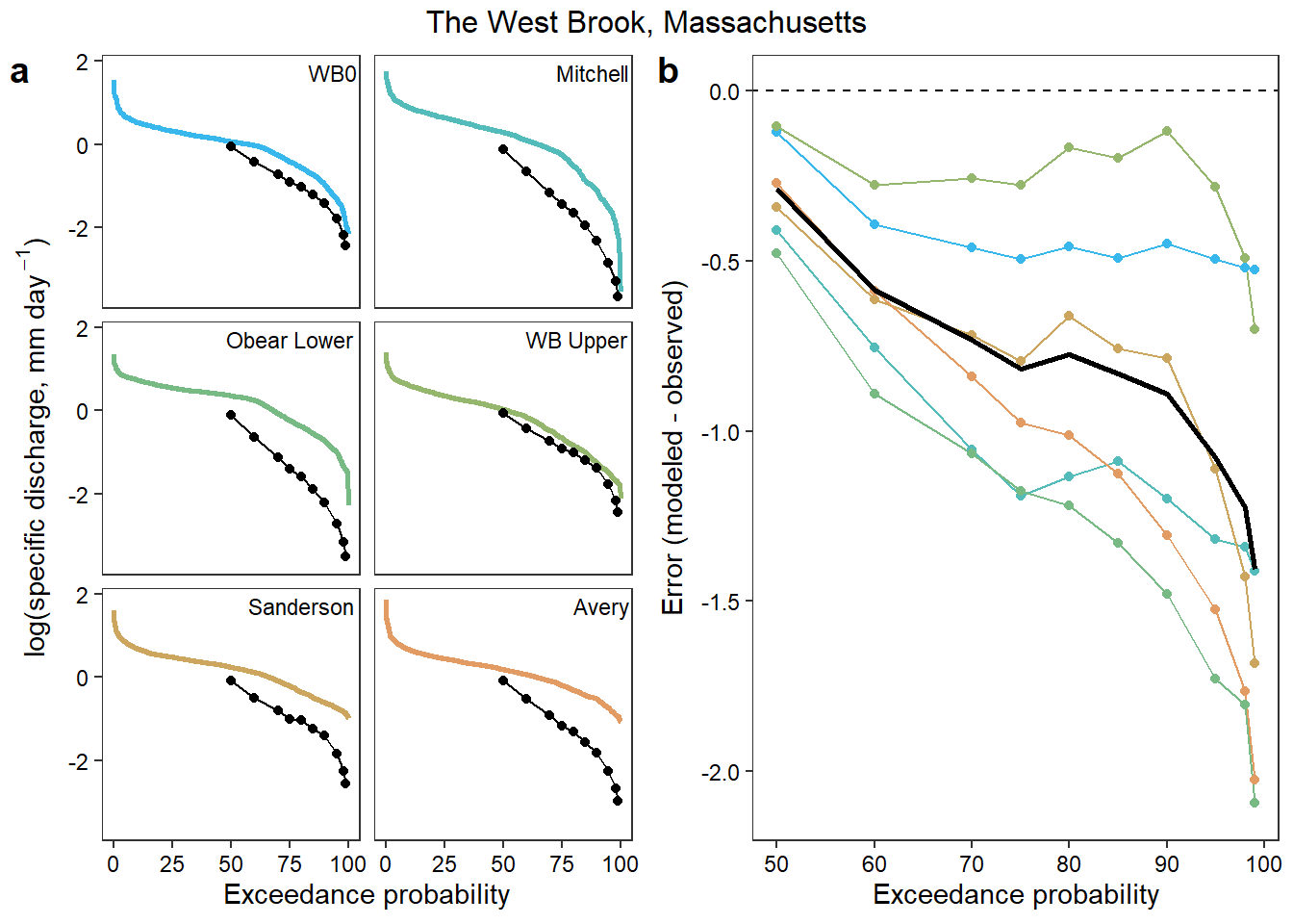
### No Color
# exceedance curves
p1 <- ggplot() +
geom_line(data = exceed, aes(x = exceedance, y = logYield), size = 1) +
geom_line(data = preds, aes(x = exceedance, y = logYield), color = "red") +
geom_point(data = preds, aes(x = exceedance, y = logYield), color = "red") +
geom_text(data = siteslabs, aes(x = Inf, y = Inf, label = site_name), vjust = 1.5, hjust = 1.05, size = 3) +
facet_wrap(~site_name, nrow = 3) +
xlab("Exceedance probability") + ylab("log(Yield, mm)") +
theme_bw() + theme(panel.grid.major = element_blank(), panel.grid.minor = element_blank(),
panel.grid = element_blank(), strip.text.x = element_blank(), strip.background = element_blank(),
legend.position = "none")
# absolute error
p2 <- ggplot(data = joined) +
geom_line(aes(x = exceedance, y = error_abs, group = site_name)) +
geom_point(aes(x = exceedance, y = error_abs, group = site_name)) +
geom_abline(intercept = 0, slope = 0, linetype = "dashed") +
geom_line(data = joined_mean, aes(x = exceedance, y = error_abs), size = 1, col = "red") +
xlab("Exceedance probability") + ylab("Absolute error") + ylim(-2.1,0) +
theme_bw() + theme(panel.grid.major = element_blank(), panel.grid.minor = element_blank(),
legend.position = "none")
# combine
annotate_figure(ggarrange(p1, p2, ncol = 2, labels = "auto"), top = text_grob("The West Brook, Massachusetts"))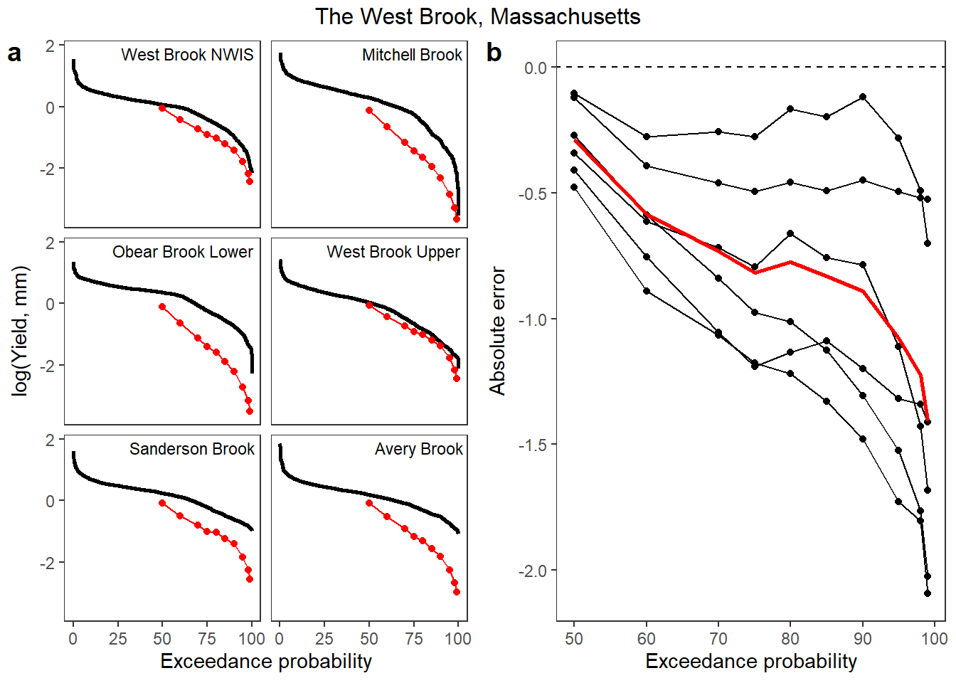
Does StreamStats misrepresent among-site variation in flow duration?
p1 <- ggplot() +
geom_line(data = vardat_obs, aes(x = exceedance, y = exdsd), size = 1, color = "grey60") +
geom_line(data = vardat_ss, aes(x = exceedance, y = exdsd), color = "black") +
geom_point(data = vardat_ss, aes(x = exceedance, y = exdsd), color = "black") +
xlab("Exceedance probability") + ylab("Among-site standard deviation in log(Yield, mm)") +
theme_bw() + theme(panel.grid.major = element_blank(), panel.grid.minor = element_blank())
p2 <- vardat_obs %>%
left_join(vardat_ss %>% rename(exdsd_ss = exdsd)) %>%
mutate(diff = exdsd_ss - exdsd) %>%
filter(!is.na(diff)) %>%
ggplot() +
geom_line(aes(x = exceedance, y = diff)) +
geom_abline(intercept = 0, slope = 0, linetype = "dashed") +
xlab("Exceedance probability") + ylab("Difference") +
theme_bw() + theme(panel.grid.major = element_blank(), panel.grid.minor = element_blank())
annotate_figure(ggarrange(p1, p2, ncol = 2, labels = "auto"), top = text_grob("The West Brook, Massachusetts"))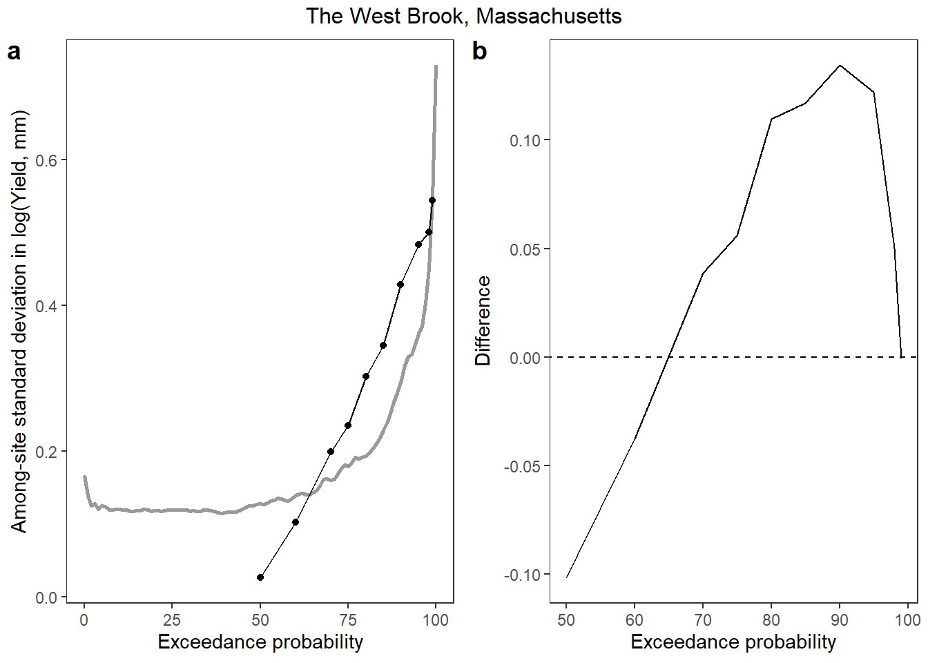
Write to file
mypal <- cet_pal(length(wborder), name = "i1")[c(1,3,5,6,8,9)]
### Colored by site
# exceedance curves
p1 <- ggplot() +
geom_line(data = exceed, aes(x = exceedance, y = logYield, color = site_name), size = 1) +
geom_line(data = preds, aes(x = exceedance, y = logYield), color = "black") +
geom_point(data = preds, aes(x = exceedance, y = logYield), color = "black") +
geom_text(data = siteslabs, aes(x = Inf, y = Inf, label = site_lab), vjust = 1.5, hjust = 1.05, size = 3) +
facet_wrap(~site_name, nrow = 3) +
scale_color_manual(values = mypal) +
xlab("Exceedance probability") + ylab(expression(paste("log(specific discharge, mm day"^-1, ")", sep = ""))) +
theme_bw() + theme(panel.grid.major = element_blank(), panel.grid.minor = element_blank(),
panel.grid = element_blank(), strip.text.x = element_blank(), strip.background = element_blank(),
legend.position = "none", axis.text = element_text(color = "black"))
# absolute error
p2 <- ggplot(data = joined) +
geom_line(aes(x = exceedance, y = error_abs, group = site_name, color = site_name)) +
geom_point(aes(x = exceedance, y = error_abs, group = site_name, color = site_name)) +
geom_abline(intercept = 0, slope = 0, linetype = "dashed") +
geom_line(data = joined_mean, aes(x = exceedance, y = error_abs), size = 1) +
scale_color_manual(values = mypal) +
xlab("Exceedance probability") + ylab("Error (modeled - observed)") + ylim(-2.1,0) +
theme_bw() + theme(panel.grid.major = element_blank(), panel.grid.minor = element_blank(),
legend.position = "none", axis.text = element_text(color = "black"))
# combine
jpeg("C:/Users/jbaldock/OneDrive - DOI/Documents/USGS/EcoDrought/EcoDrought Working/Presentation figs/StreamStats_WestBrook.jpg", width = 6, height = 4, units = "in", res = 1000)
annotate_figure(ggarrange(p1, p2, ncol = 2, labels = "auto"), top = text_grob("The West Brook, Massachusetts"))
dev.off()For the Flathead (Big Creek), plot observed and StreamStats mean monthly flow/yield and calculate absolute error
# set up
vars <- unique(montana$StatName)[grep("Mean Flow", unique(montana$StatName))]
sites <- c("LangfordCreekUpper", "Big Creek NWIS", "HallowattCreekLower", "WernerCreek", "Hallowat Creek NWIS", "McGeeCreekLower")
preds_list <- list()
obs_list <- list()
hull_list <- list()
join_list <- list()
# calcualate
for (i in 1:length(sites)) {
# filter observed data
obs <- dat_clean %>%
filter(site_name == sites[i]) %>%
mutate(MonthName = factor(MonthName, levels = c("Oct", "Nov", "Dec", "Jan", "Feb", "Mar", "Apr", "May", "Jun", "Jul", "Aug", "Sep")))
# calculate monthly means
obs_mon <- obs %>%
group_by(site_name, WaterYear, MonthName) %>%
summarize(logYield = mean(logYield)) %>%
ungroup() %>%
mutate(MonthName = factor(MonthName, levels = c("Oct", "Nov", "Dec", "Jan", "Feb", "Mar", "Apr", "May", "Jun", "Jul", "Aug", "Sep")),
WaterYear = factor(WaterYear)) %>%
complete(site_name, WaterYear, MonthName)
# get monthly min/max for ribbon
hull <- obs_mon %>%
group_by(site_name, MonthName) %>%
summarize(min_logYield = min(logYield, na.rm = TRUE), max_logYield = max(logYield, na.rm = TRUE)) %>%
ungroup()
# get StreamStats mean monthly flow
preds <- streamstats %>%
filter(site_name == sites[i], StatName %in% vars, !is.na(AreaSqMi)) %>%
mutate(MonthName = substr(StatName, 1, nchar(StatName)-10),
Month = parse_number(StatLabel)) %>%
mutate(MonthName = factor(recode(MonthName, "January" = "Jan", "February" = "Feb", "March" = "Mar", "April" = "Apr", "June" = "Jun", "July" = "Jul", "August" = "Aug", "September" = "Sep", "October" = "Oct", "November" = "Nov", "December" = "Dec"), levels = c("Oct", "Nov", "Dec", "Jan", "Feb", "Mar", "Apr", "May", "Jun", "Jul", "Aug", "Sep"))) %>%
mutate(flow_cms = Value*0.02831683199881, area_sqkm = AreaSqMi*2.58999)
preds <- add_daily_yield(data = preds %>% select(site_id, site_name, area_sqkm, MonthName, Month, flow_cms), values = flow_cms, basin_area = as.numeric(unique(preds$area_sqkm)))
preds <- preds %>% mutate(logYield = log(Yield_mm))
# join and calculate error
join_list[[i]] <- obs_mon %>%
left_join(preds %>% select(site_name, MonthName, logYield) %>% rename(logYield_ss = logYield)) %>%
mutate(error_abs = logYield_ss - logYield,
error_abs_real = exp(logYield_ss) - exp(logYield),
error_rel = (exp(logYield_ss) - exp(logYield)) / exp(logYield))
# store in list
preds_list[[i]] <- preds
obs_list[[i]] <- obs_mon
hull_list[[i]] <- hull
}
preds <- do.call(rbind, preds_list) %>% mutate(site_name = factor(site_name, levels = flatorder))
obs_mon <- do.call(rbind, obs_list) %>% mutate(site_name = factor(site_name, levels = flatorder))
hull <- do.call(rbind, hull_list) %>% mutate(site_name = factor(site_name, levels = flatorder))
joined <- do.call(rbind, join_list) %>% mutate(site_name = factor(site_name, levels = flatorder))
joined_mean <- joined %>% group_by(MonthName) %>% summarise(error_abs = mean(error_abs, na.rm = TRUE))
# tibble for site labels
siteslabs <- tibble(site_name = factor(sites, levels = flatorder), site_lab = c("Langford", "Big", "Hallowatt Lower", "Werner", "Hallowatt Upper", "McGee"))
# calculate among site variation for StreamStats and observed mean monthly flow (mean across years)
vardat <- preds %>%
group_by(MonthName) %>%
summarize(qsd_ss = sd(logYield)) %>%
ungroup() %>%
left_join(obs_mon %>%
group_by(site_name, MonthName) %>%
summarize(logYield = mean(logYield, na.rm = TRUE)) %>%
ungroup() %>%
group_by(MonthName) %>%
summarize(qsd_obs = sd(logYield)) %>%
ungroup()) %>%
mutate(diff = qsd_ss - qsd_obs, nummon = as.numeric(MonthName))mypal <- cet_pal(length(flatorder), name = "i1")[c(3,4,6,8,9,17)]
### Colored by site
# observed and StreamStats monthly flow
p1 <- ggplot() +
geom_ribbon(data = hull, aes(ymin = min_logYield, ymax = max_logYield, x = as.numeric(MonthName), fill = site_name), alpha = 0.3) +
geom_line(data = obs_mon, aes(y = logYield, x = as.numeric(MonthName), group = WaterYear, color = site_name)) +
geom_point(data = obs_mon, aes(y = logYield, x = as.numeric(MonthName), group = WaterYear, shape = WaterYear, color = site_name)) +
geom_line(data = preds, aes(y = logYield, x = as.numeric(MonthName), group = site_name), color = "black") +
geom_point(data = preds, aes(y = logYield, x = as.numeric(MonthName)), color = "black") +
geom_text(data = siteslabs, aes(x = -Inf, y = Inf, label = site_lab), vjust = 1.5, hjust = -0.05, size = 3) +
facet_wrap(~site_name, ncol = 2) +
scale_color_manual(values = mypal) +
scale_fill_manual(values = mypal) +
theme_bw() + theme(panel.grid.major = element_blank(), panel.grid.minor = element_blank(), legend.position = "none",
strip.text.x = element_blank(), strip.background = element_blank()) +
ylab(expression(paste("Monthly mean log(specific discharge, mm day"^-1, ")", sep = ""))) + xlab("Month") +
scale_x_continuous(breaks = 1:12, labels = c("O", "N", "D", "J", "F", "M", "A", "M", "J", "J", "A", "S"))
# absolute error by month
p2 <- ggplot() +
geom_line(data = joined, aes(x = as.numeric(MonthName), y = error_abs, shape = WaterYear, color = site_name)) +
geom_point(data = joined, aes(x = as.numeric(MonthName), y = error_abs, shape = WaterYear, color = site_name)) +
geom_line(data = joined_mean, aes(x = as.numeric(MonthName), y = error_abs), size = 1) +
geom_abline(intercept = 0, slope = 0, linetype = "dashed") +
scale_color_manual(values = mypal) +
xlab("Month") + ylab("Error (modeled - observed)") +
scale_x_continuous(breaks = 1:12, labels = c("O", "N", "D", "J", "F", "M", "A", "M", "J", "J", "A", "S")) +
theme_bw() + theme(panel.grid.major = element_blank(), panel.grid.minor = element_blank(),
legend.position = "none")
# combine
annotate_figure(ggarrange(p1, p2, ncol = 2, labels = "auto"), top = text_grob("North Fork Flathead River, Montana"))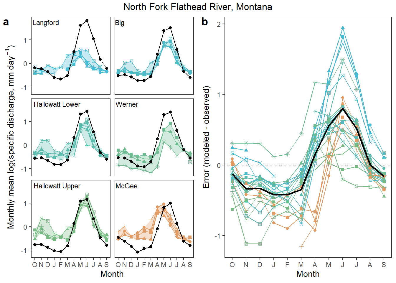
### No color
# observed and StreamStats monthly flow
p1 <- ggplot() +
geom_ribbon(data = hull, aes(ymin = min_logYield, ymax = max_logYield, x = as.numeric(MonthName)), fill = "grey80") +
geom_line(data = obs_mon, aes(y = logYield, x = as.numeric(MonthName), group = WaterYear)) +
geom_point(data = obs_mon, aes(y = logYield, x = as.numeric(MonthName), group = WaterYear, shape = WaterYear)) +
geom_line(data = preds, aes(y = logYield, x = as.numeric(MonthName), group = site_name), color = "red") +
geom_point(data = preds, aes(y = logYield, x = as.numeric(MonthName)), color = "red") +
geom_text(data = siteslabs, aes(x = -Inf, y = Inf, label = site_lab), vjust = 1.5, hjust = -0.05, size = 3) +
facet_wrap(~site_name, ncol = 2) +
theme_bw() + theme(panel.grid.major = element_blank(), panel.grid.minor = element_blank(), legend.position = "none",
strip.text.x = element_blank(), strip.background = element_blank()) +
ylab(expression(paste("Monthly mean log(specific discharge, mm day"^-1, ")", sep = ""))) + xlab("Month") +
scale_x_continuous(breaks = 1:12, labels = c("O", "N", "D", "J", "F", "M", "A", "M", "J", "J", "A", "S"))
# absolute error by month
p2 <- ggplot() +
geom_line(data = joined, aes(x = as.numeric(MonthName), y = error_abs, group = interaction(site_name, WaterYear))) +
geom_point(data = joined, aes(x = as.numeric(MonthName), y = error_abs, shape = WaterYear)) +
geom_line(data = joined_mean, aes(x = as.numeric(MonthName), y = error_abs), size = 1, col = "red") +
geom_abline(intercept = 0, slope = 0, linetype = "dashed") +
xlab("Month") + ylab("Absolute error") +
scale_x_continuous(breaks = 1:12, labels = c("O", "N", "D", "J", "F", "M", "A", "M", "J", "J", "A", "S")) +
theme_bw() + theme(panel.grid.major = element_blank(), panel.grid.minor = element_blank(),
legend.position = "none")
# combine
annotate_figure(ggarrange(p1, p2, ncol = 2, labels = "auto"), top = text_grob("North Fork Flathead River, Montana"))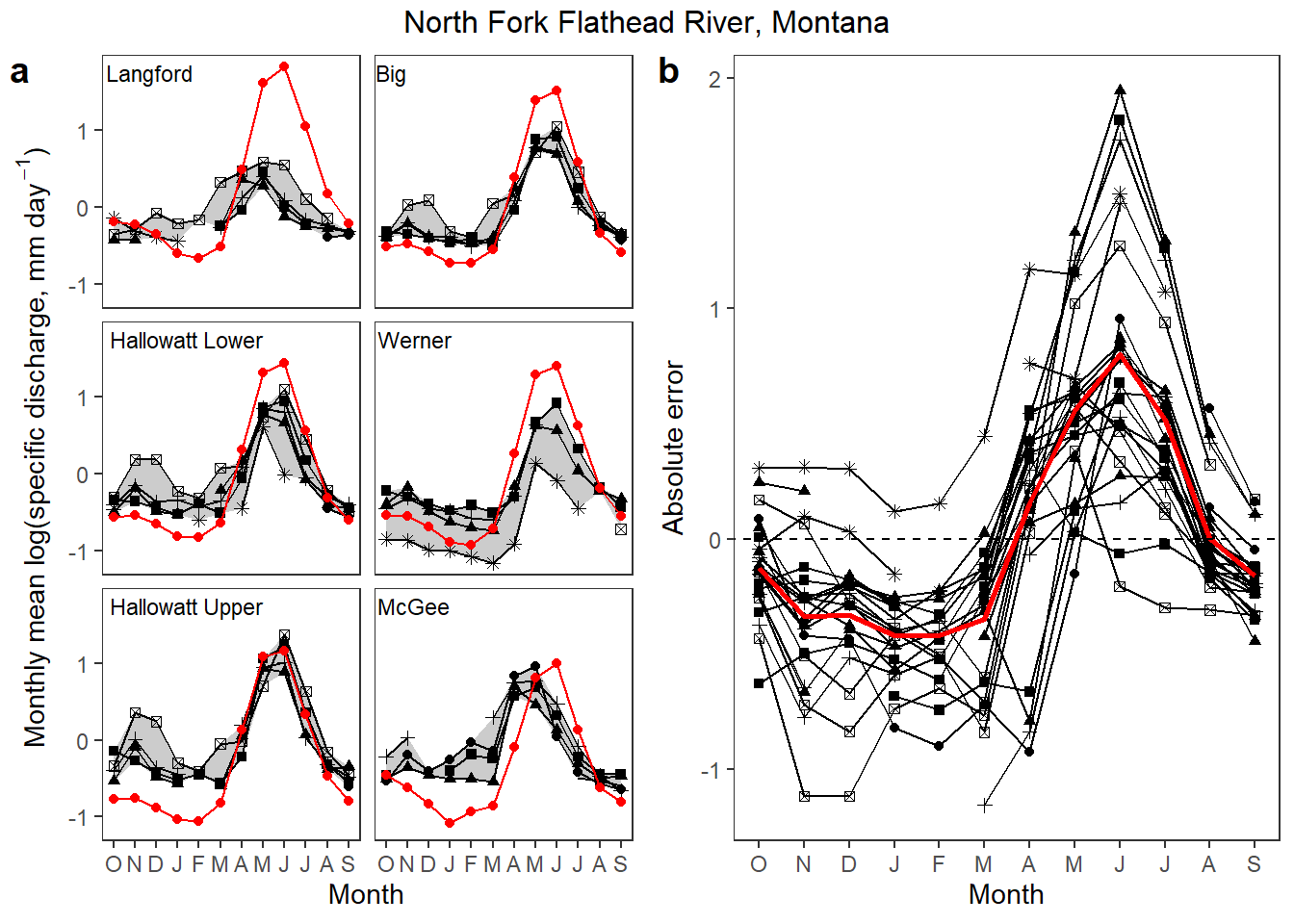
Does StreamStats misrepresent among-site variation in mean monthly yield?
p1 <- vardat %>%
ggplot() +
geom_line(aes(x = nummon, y = qsd_obs), size = 1, color = "grey60") +
geom_line(aes(x = nummon, y = qsd_ss), color = "black") +
geom_point(aes(x = nummon, y = qsd_ss), color = "black") +
xlab("Month") + ylab("Among-site standard deviation in log(Yield, mm)") +
scale_x_continuous(breaks = 1:12, labels = c("O", "N", "D", "J", "F", "M", "A", "M", "J", "J", "A", "S")) +
theme_bw() + theme(panel.grid.major = element_blank(), panel.grid.minor = element_blank())
p2 <- vardat %>%
ggplot() +
geom_line(aes(x = nummon, y = diff)) +
xlab("Month") + ylab("Difference") +
geom_abline(intercept = 0, slope = 0, linetype = "dashed") +
scale_x_continuous(breaks = 1:12, labels = c("O", "N", "D", "J", "F", "M", "A", "M", "J", "J", "A", "S")) +
theme_bw() + theme(panel.grid.major = element_blank(), panel.grid.minor = element_blank())
annotate_figure(ggarrange(p1, p2, ncol = 2, labels = "auto"), top = text_grob("North Fork Flathead River, Montana"))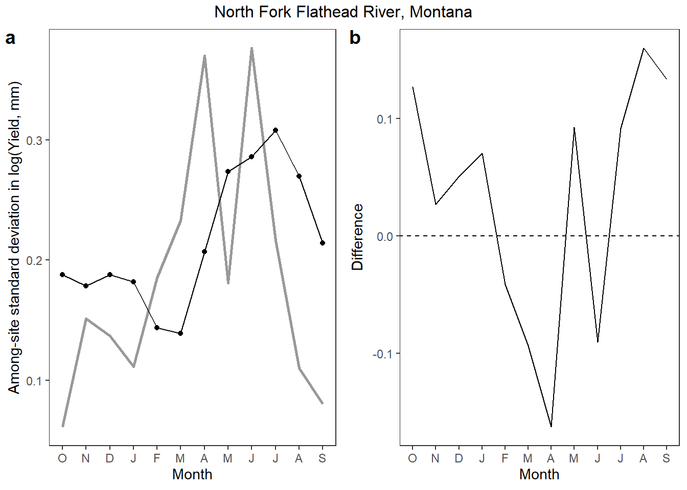
Write to file
mypal <- cet_pal(length(flatorder), name = "i1")[c(3,4,6,8,9,17)]
### Colored by site
# observed and StreamStats monthly flow
p1 <- ggplot() +
geom_ribbon(data = hull, aes(ymin = min_logYield, ymax = max_logYield, x = as.numeric(MonthName), fill = site_name), alpha = 0.3) +
geom_line(data = obs_mon, aes(y = logYield, x = as.numeric(MonthName), group = WaterYear, color = site_name)) +
geom_point(data = obs_mon, aes(y = logYield, x = as.numeric(MonthName), group = WaterYear, shape = WaterYear, color = site_name)) +
geom_line(data = preds, aes(y = logYield, x = as.numeric(MonthName), group = site_name), color = "black") +
geom_point(data = preds, aes(y = logYield, x = as.numeric(MonthName)), color = "black") +
geom_text(data = siteslabs, aes(x = -Inf, y = Inf, label = site_lab), vjust = 1.5, hjust = -0.05, size = 3) +
facet_wrap(~site_name, ncol = 2) +
scale_color_manual(values = mypal) +
scale_fill_manual(values = mypal) +
theme_bw() + theme(panel.grid.major = element_blank(), panel.grid.minor = element_blank(), legend.position = "none",
strip.text.x = element_blank(), strip.background = element_blank()) +
ylab(expression(paste("Monthly mean log(specific discharge, mm day"^-1, ")", sep = ""))) + xlab("Month") +
scale_x_continuous(breaks = 1:12, labels = c("O", "N", "D", "J", "F", "M", "A", "M", "J", "J", "A", "S"))
# absolute error by month
p2 <- ggplot() +
geom_line(data = joined, aes(x = as.numeric(MonthName), y = error_abs, shape = WaterYear, color = site_name)) +
geom_point(data = joined, aes(x = as.numeric(MonthName), y = error_abs, shape = WaterYear, color = site_name)) +
geom_line(data = joined_mean, aes(x = as.numeric(MonthName), y = error_abs), size = 1) +
geom_abline(intercept = 0, slope = 0, linetype = "dashed") +
scale_color_manual(values = mypal) +
xlab("Month") + ylab("Error (modeled - observed)") +
scale_x_continuous(breaks = 1:12, labels = c("O", "N", "D", "J", "F", "M", "A", "M", "J", "J", "A", "S")) +
theme_bw() + theme(panel.grid.major = element_blank(), panel.grid.minor = element_blank(),
legend.position = "none")
# combine
jpeg("C:/Users/jbaldock/OneDrive - DOI/Documents/USGS/EcoDrought/EcoDrought Working/Presentation figs/StreamStats_Flathead.jpg", width = 6, height = 4, units = "in", res = 1000)
annotate_figure(ggarrange(p1, p2, ncol = 2), top = text_grob("North Fork Flathead River, Montana"))
dev.off()Pull streamflow predictions from Montana Climate Office’s (University of Montana) Streamflow API. The finest spatial resolution of streamflow predictions is HUC-10. This means that all sites within subbasins have the same predicted streamflow. This makes we wonder how relevant/useful these comparisons are, beyond g/G comparisons shown for objective 1.
Get HUC-10 watershed codes
myhucs <- c()
for (i in 1:dim(siteinfo_sp)[1]) { myhucs[i] <- get_huc(AOI = siteinfo_sp[i,], type = "huc10")$huc10 }
siteinfo <- siteinfo %>% mutate(huc10 = myhucs)
myhucs <- unique(myhucs)
#length(myhucs)Query UM Climatology
request = httr::GET(
# can replace this with /predictions/raw, the only query parameter that isn't shared is aggregations.
"https://data.climate.umt.edu/streamflow-api/predictions/",
query = list(
locations = paste(myhucs, collapse = ","),
date_start = "2015-01-01",
date_end = "2025-01-01",
aggregations = "mean",
as_csv = TRUE,
units = "mm"
)
)
umpreds <- httr::content(request)
umpreds <- umpreds %>% rename(huc10 = location)
print(umpreds)
write_csv(umpreds, "C:/Users/jbaldock/OneDrive - DOI/Documents/USGS/EcoDrought/EcoDrought Working/EcoDrought-Analysis/CompareModeledQ/UM_Climatology_PredictedQ.shp")Load UM Climatrology predicted flow data
umpreds <- read_csv("C:/Users/jbaldock/OneDrive - DOI/Documents/USGS/EcoDrought/EcoDrought Working/EcoDrought-Analysis/CompareModeledQ/UM_Climatology_PredictedQ.shp")
umpreds# A tibble: 58,464 × 5
huc10 version date metric value
<chr> <chr> <date> <chr> <dbl>
1 0108020106 vPUB2025 2015-01-01 mean 2.14
2 0108020106 vPUB2025 2015-01-02 mean 1.86
3 0108020106 vPUB2025 2015-01-03 mean 1.93
4 0108020106 vPUB2025 2015-01-04 mean 4.00
5 0108020106 vPUB2025 2015-01-05 mean 4.04
6 0108020106 vPUB2025 2015-01-06 mean 3.07
7 0108020106 vPUB2025 2015-01-07 mean 2.43
8 0108020106 vPUB2025 2015-01-08 mean 2.16
9 0108020106 vPUB2025 2015-01-09 mean 2.03
10 0108020106 vPUB2025 2015-01-10 mean 1.90
# ℹ 58,454 more rowsJoin to observed data
dat_umpred <- dat_clean %>%
left_join(siteinfo %>% select(site_name, huc10)) %>%
left_join(umpreds %>% select(huc10, date, value)) Plot all time series data
umpreds %>%
ggplot(aes(x = date, y = value)) +
geom_line() +
facet_wrap(~huc10, scales = "free_y")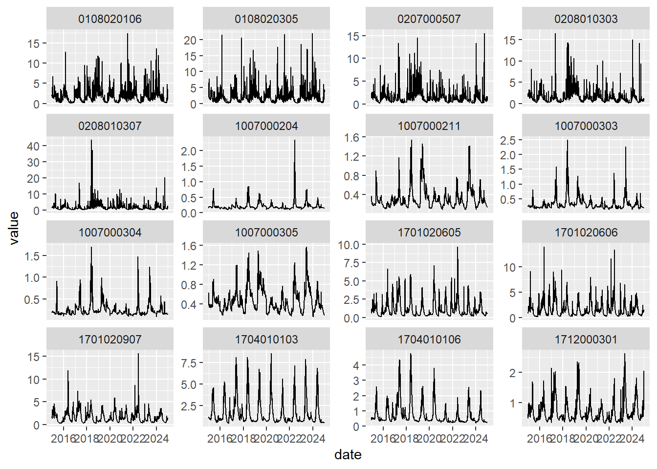
Compare predicted (red) and observed (black) streamflow data for select sites/basins. For some sites, modeled flow captures the general patterns/shapes of observed hydrographs well, but accuracy is reduced at fine temporal resolutions. For other sites, modeled flow fails to capture both the general and finer resolution asepcts of observed data.
dat_umpred %>% filter(site_name == "Jimmy Brook") %>% select(date, Yield_mm, value) %>% dygraph() %>% dySeries("Yield_mm", color = "black") %>% dySeries("value", color = "red") %>% dyRangeSelector() %>% dyAxis("y", label = "Yield (mm)") dat_umpred %>% filter(site_name == "Staunton River 06") %>% select(date, Yield_mm, value) %>% dygraph() %>% dySeries("Yield_mm", color = "black") %>% dySeries("value", color = "red") %>% dyRangeSelector() %>% dyAxis("y", label = "Yield (mm)") dat_umpred %>% filter(site_name == "Hallowat Creek NWIS") %>% select(date, Yield_mm, value) %>% dygraph() %>% dySeries("Yield_mm", color = "black") %>% dySeries("value", color = "red") %>% dyRangeSelector() %>% dyAxis("y", label = "Yield (mm)") dat_umpred %>% filter(site_name == "SF Spread Creek Lower") %>% select(date, Yield_mm, value) %>% dygraph() %>% dySeries("Yield_mm", color = "black") %>% dySeries("value", color = "red") %>% dyRangeSelector() %>% dyAxis("y", label = "Yield (mm)") dat_umpred %>% filter(site_name == "Dugout Creek") %>% select(date, Yield_mm, value) %>% dygraph() %>% dySeries("Yield_mm", color = "black") %>% dySeries("value", color = "red") %>% dyRangeSelector() %>% dyAxis("y", label = "Yield (mm)") dat_umpred %>% filter(site_name == "Donner Blitzen ab Indian NWIS") %>% select(date, Yield_mm, value) %>% dygraph() %>% dySeries("Yield_mm", color = "black") %>% dySeries("value", color = "red") %>% dyRangeSelector() %>% dyAxis("y", label = "Yield (mm)") NSE scores and categories per Moriasi et al. “Model evaluation guidelines for systematic quantification of accuracy in watershed simulations.” Transactions of the ASABE 50.3 (2007): 885-900.
| Category | NSE range |
|---|---|
| Very good | 0.75-1.00 |
| Good | 0.65-0.75 |
| Satisfactory | 0.50-0.65 |
| Unsatisfactory | <0.50 |
Note that there is no effort to ensure consistant data availability among sites/basins/years. Would it be better to restrict these?
NSE by subbasin for all available data.
dat_umpred %>%
group_by(site_name, subbasin) %>%
summarize(nse = NSE(sim = log(value), obs = log(Yield_mm))) %>%
ungroup() %>%
mutate(subbasin = factor(subbasin, levels = c("West Brook", "Paine Run", "Staunton River", "Big Creek", "Coal Creek", "McGee Creek", "Snake River", "Shields River", "Duck Creek", "Donner Blitzen"))) %>%
ggplot(aes(x = subbasin, y = nse)) +
annotate("rect", xmin = -Inf, xmax = Inf, ymin = -Inf, ymax = 0.50, alpha = 0.3, fill = "red") +
annotate("rect", xmin = -Inf, xmax = Inf, ymin = 0.50, ymax = 0.65, alpha = 0.3, fill = "orange") +
annotate("rect", xmin = -Inf, xmax = Inf, ymin = 0.65, ymax = 0.75, alpha = 0.3, fill = "yellow") +
annotate("rect", xmin = -Inf, xmax = Inf, ymin = 0.75, ymax = 1.00, alpha = 0.3, fill = "green") +
geom_boxplot(fill = "grey", outlier.shape = NA) +
geom_jitter(height = 0, width = 0.2, shape = 1) +
geom_abline(slope = 0, intercept = 1, color = "black", linetype = "dashed") +
xlab("Sub-basin") + ylab("Nash-Sutcliffe efficiency") + ggtitle("All data") +
theme_bw() +
theme(panel.grid.major = element_blank(), panel.grid.minor = element_blank(),
axis.text.x = element_text(angle = 45, vjust = 0.5, hjust = 0.4)) +
scale_y_continuous(limits = c(-8.5,1), expand = c(0,0))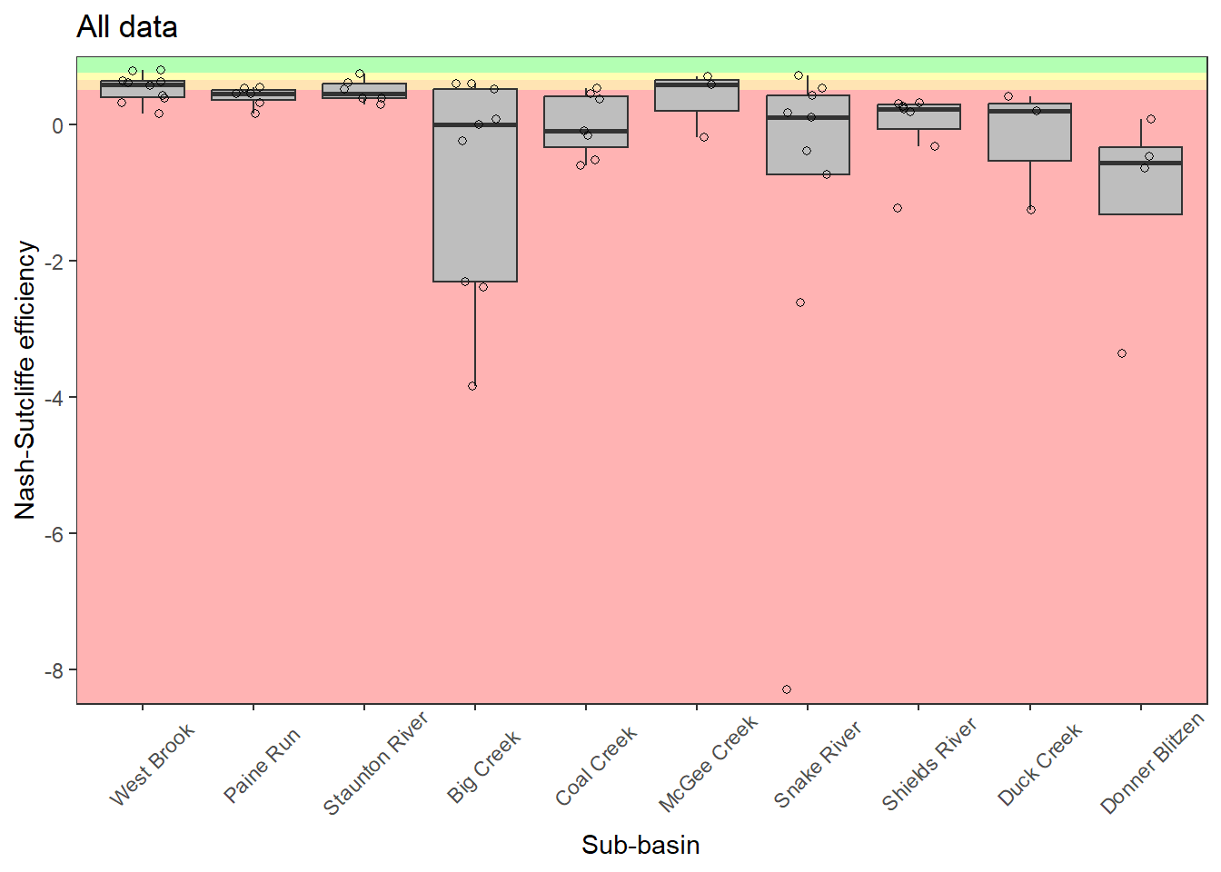
NSE by subbasin, summer (July-August) only, all available years.
dat_umpred %>%
filter(Month %in% c(7:9)) %>%
group_by(site_name, subbasin) %>%
summarize(nse = NSE(sim = log(value), obs = log(Yield_mm))) %>%
ungroup() %>%
mutate(subbasin = factor(subbasin, levels = c("West Brook", "Paine Run", "Staunton River", "Big Creek", "Coal Creek", "McGee Creek", "Snake River", "Shields River", "Duck Creek", "Donner Blitzen"))) %>%
ggplot(aes(x = subbasin, y = nse)) +
annotate("rect", xmin = -Inf, xmax = Inf, ymin = -Inf, ymax = 0.50, alpha = 0.3, fill = "red") +
annotate("rect", xmin = -Inf, xmax = Inf, ymin = 0.50, ymax = 0.65, alpha = 0.3, fill = "orange") +
annotate("rect", xmin = -Inf, xmax = Inf, ymin = 0.65, ymax = 0.75, alpha = 0.3, fill = "yellow") +
annotate("rect", xmin = -Inf, xmax = Inf, ymin = 0.75, ymax = 1.00, alpha = 0.3, fill = "green") +
geom_boxplot(fill = "grey", outlier.shape = NA) +
geom_jitter(height = 0, width = 0.2, shape = 1) +
geom_abline(slope = 0, intercept = 1, color = "black", linetype = "dashed") +
xlab("Sub-basin") + ylab("Nash-Sutcliffe efficiency") + ggtitle("July-September") +
theme_bw() +
theme(panel.grid.major = element_blank(), panel.grid.minor = element_blank(),
axis.text.x = element_text(angle = 45, vjust = 0.5, hjust = 0.4)) +
scale_y_continuous(limits = c(-12.5,1), expand = c(0,0))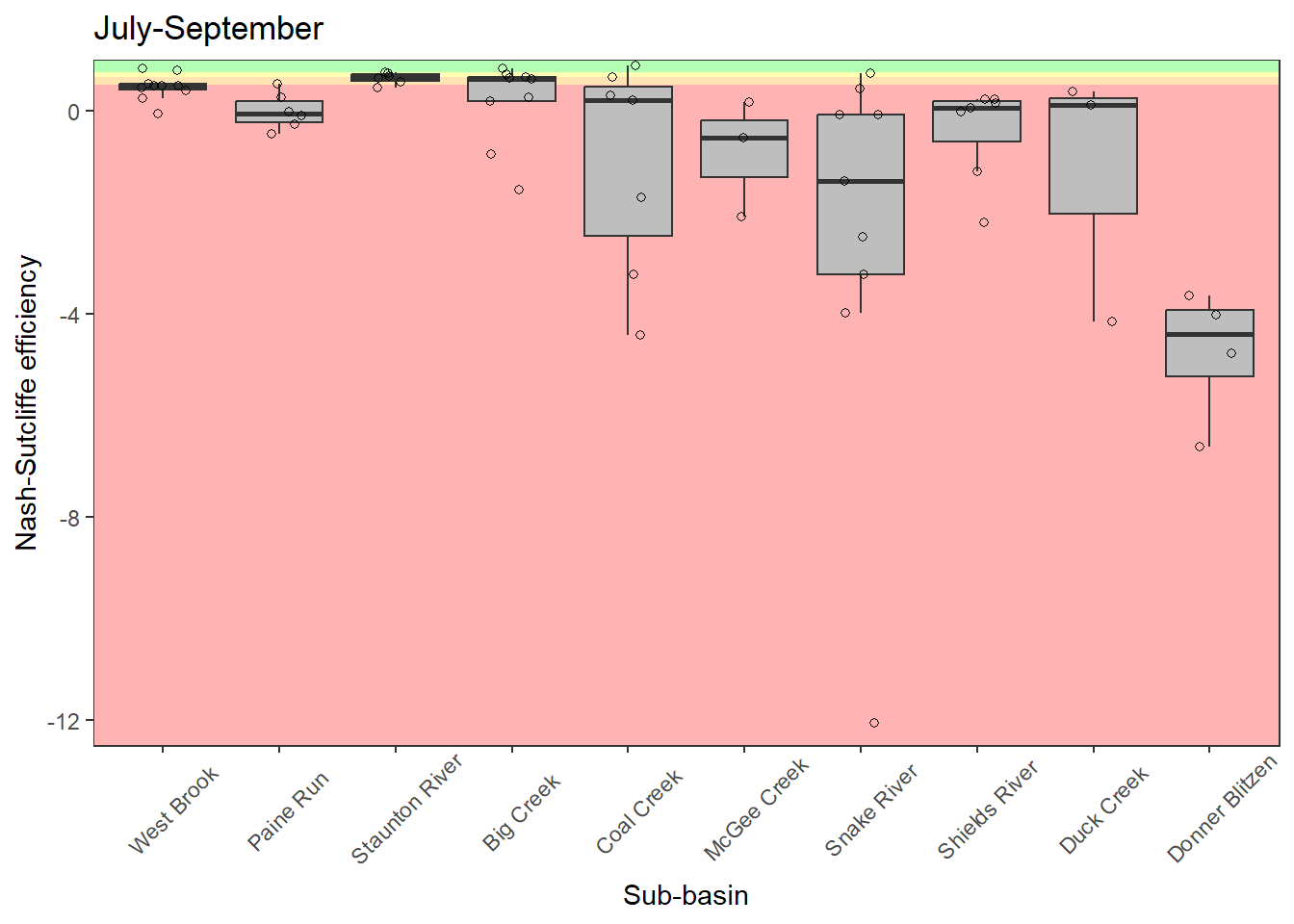
How does NSE vary through time?
NSE by subbasin and month, pooled across all available years
dat_umpred %>%
group_by(site_name, subbasin, MonthName) %>%
summarize(nse = NSE(sim = log(value), obs = log(Yield_mm))) %>%
ungroup() %>%
mutate(subbasin = factor(subbasin, levels = c("West Brook", "Paine Run", "Staunton River", "Big Creek", "Coal Creek", "McGee Creek", "Snake River", "Shields River", "Duck Creek", "Donner Blitzen")),
MonthName = factor(MonthName, levels = c("Jan", "Feb", "Mar", "Apr", "May", "Jun", "Jul", "Aug", "Sep", "Oct", "Nov", "Dec"))) %>%
ggplot(aes(x = MonthName, y = nse)) +
annotate("rect", xmin = -Inf, xmax = Inf, ymin = -Inf, ymax = 0.50, alpha = 0.3, fill = "red") +
annotate("rect", xmin = -Inf, xmax = Inf, ymin = 0.50, ymax = 0.65, alpha = 0.3, fill = "orange") +
annotate("rect", xmin = -Inf, xmax = Inf, ymin = 0.65, ymax = 0.75, alpha = 0.3, fill = "yellow") +
annotate("rect", xmin = -Inf, xmax = Inf, ymin = 0.75, ymax = 1.00, alpha = 0.3, fill = "green") +
geom_point(aes(group = site_name)) +
geom_abline(slope = 0, intercept = 1, color = "black", linetype = "dashed") +
scale_x_discrete(labels = c("Jan" = "J", "Feb" = "F", "Mar" = "M", "Apr" = "A", "May" = "M", "Jun" = "J", "Jul" = "J", "Aug" = "A", "Sep" = "S", "Oct" = "O", "Nov" = "N", "Dec" = "D")) +
xlab("Month") + ylab("Nash-Sutcliffe efficiency") + ggtitle("All data") +
facet_wrap(~subbasin, scales = "free_y") +
theme_bw() +
theme(panel.grid.major = element_blank(), panel.grid.minor = element_blank()) +
scale_y_continuous(expand = c(0,0))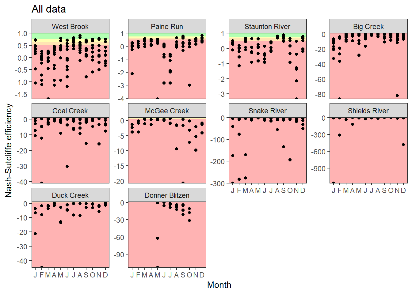
For the West Brook, show NSE by time and site, no pooling.
dat_umpred %>%
mutate(yearmonth = floor_date(date, "month")) %>%
filter(subbasin == "West Brook") %>%
group_by(site_name, subbasin, yearmonth) %>%
summarize(nobs = n(), nse = NSE(sim = log(value), obs = log(Yield_mm))) %>%
ungroup() %>%
filter(nobs >= 25) %>%
ggplot(aes(x = yearmonth, y = nse)) +
# annotate("rect", xmin = -Inf, xmax = Inf, ymin = -Inf, ymax = 0.50, alpha = 0.3, fill = "red") +
# annotate("rect", xmin = -Inf, xmax = Inf, ymin = 0.50, ymax = 0.65, alpha = 0.3, fill = "orange") +
# annotate("rect", xmin = -Inf, xmax = Inf, ymin = 0.65, ymax = 0.75, alpha = 0.3, fill = "yellow") +
# annotate("rect", xmin = -Inf, xmax = Inf, ymin = 0.75, ymax = 1.00, alpha = 0.3, fill = "green") +
geom_point(aes(color = site_name)) +
geom_line(aes(color = site_name)) +
geom_abline(slope = 0, intercept = 1, color = "black", linetype = "dashed") +
xlab("Time") + ylab("Nash-Sutcliffe efficiency") + ggtitle("West Brook (truncated y-axis limits)") +
#facet_wrap(~subbasin, scales = "free") +
theme_bw() +
theme(panel.grid.major = element_blank(), panel.grid.minor = element_blank()) +
ylim(-50,1)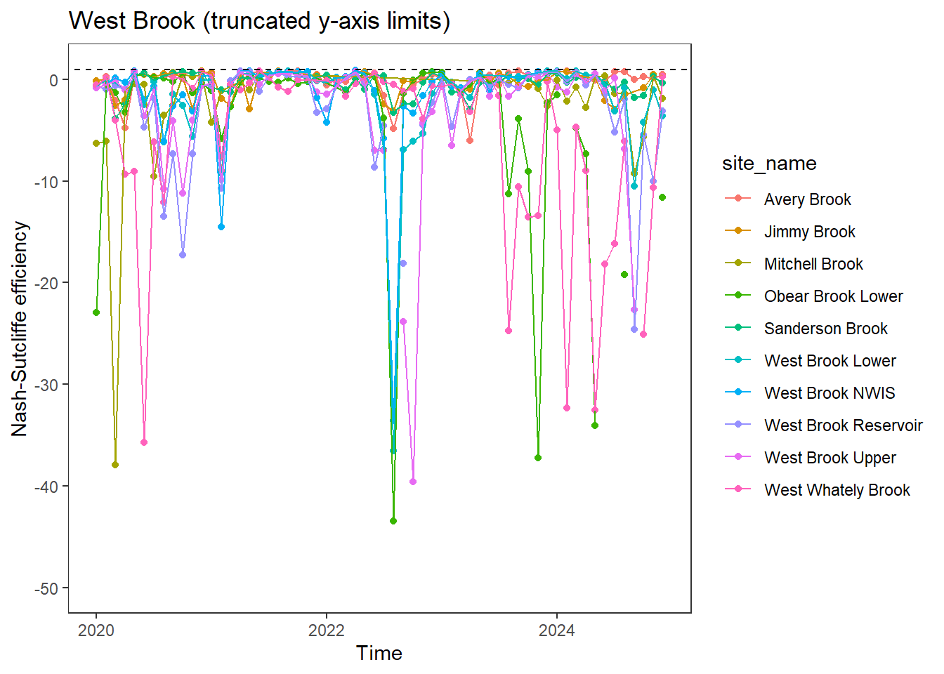
Often, ecological studyies use flow data aggregated at coarser temporal resolutions. How does efficiency change with the time scale of aggregation? Do flow predictions become more accurate when aggregated from daily to weekly or monthly means?
Aggregate data (or not), calculate NSE for each site, and combine.
daily <- dat_umpred %>%
group_by(site_name, subbasin) %>%
summarize(nse = NSE(sim = log(value), obs = log(Yield_mm))) %>%
ungroup() %>%
mutate(timescale = "day")
weekly <- dat_umpred %>%
mutate(date = floor_date(date, "week")) %>%
group_by(site_name, subbasin, date) %>%
summarise(nobs = n(), Yield_mm = mean(Yield_mm), value = mean(value)) %>%
ungroup() %>%
filter(nobs == 7) %>%
group_by(site_name, subbasin) %>%
summarize(nse = NSE(sim = log(value), obs = log(Yield_mm))) %>%
ungroup() %>%
mutate(timescale = "week")
monthly <- dat_umpred %>%
mutate(date = floor_date(date, "month")) %>%
group_by(site_name, subbasin, date) %>%
summarise(nobs = n(), Yield_mm = mean(Yield_mm), value = mean(value)) %>%
ungroup() %>%
filter(nobs >= 27) %>%
group_by(site_name, subbasin) %>%
summarize(nse = NSE(sim = log(value), obs = log(Yield_mm))) %>%
ungroup() %>%
mutate(timescale = "month")
timescale <- bind_rows(daily, weekly, monthly) %>%
mutate(timescale = factor(timescale, levels = c("day", "week", "month"))) Plot all sites
timescale %>%
ggplot(aes(x = timescale, y = nse, group = site_name)) +
annotate("rect", xmin = -Inf, xmax = Inf, ymin = -Inf, ymax = 0.50, alpha = 0.3, fill = "red") +
annotate("rect", xmin = -Inf, xmax = Inf, ymin = 0.50, ymax = 0.65, alpha = 0.3, fill = "orange") +
annotate("rect", xmin = -Inf, xmax = Inf, ymin = 0.65, ymax = 0.75, alpha = 0.3, fill = "yellow") +
annotate("rect", xmin = -Inf, xmax = Inf, ymin = 0.75, ymax = 1.00, alpha = 0.3, fill = "green") +
geom_point() +
geom_line() +
xlab("Time scale") + ylab("Nash-Sutcliffe efficiency") +
theme_bw() + ylim(-6,1) +
theme(panel.grid.major = element_blank(), panel.grid.minor = element_blank()) +
scale_y_continuous(limits = c(-14,1), expand = c(0,0))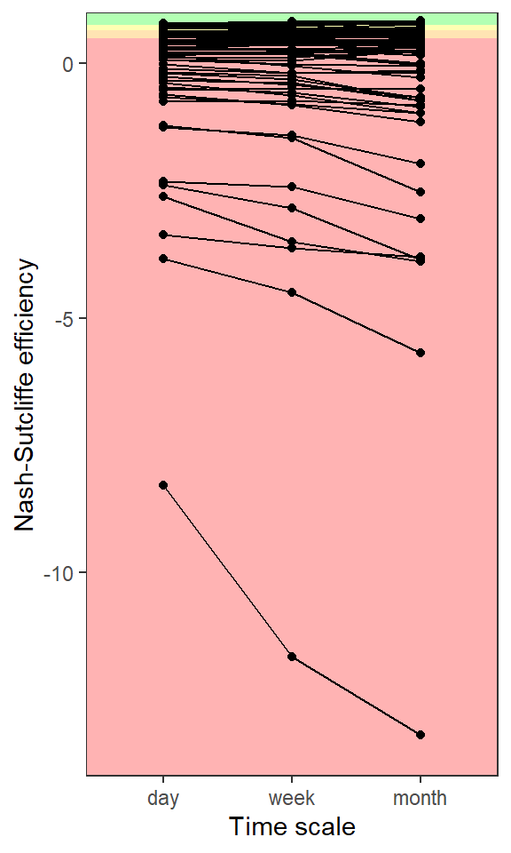
Plot all sites, facet by subbasin
timescale %>%
mutate(subbasin = factor(subbasin, levels = c("West Brook", "Paine Run", "Staunton River", "Big Creek", "Coal Creek", "McGee Creek", "Snake River", "Shields River", "Duck Creek", "Donner Blitzen"))) %>%
ggplot(aes(x = timescale, y = nse, group = site_name)) +
annotate("rect", xmin = -Inf, xmax = Inf, ymin = -Inf, ymax = 0.50, alpha = 0.3, fill = "red") +
annotate("rect", xmin = -Inf, xmax = Inf, ymin = 0.50, ymax = 0.65, alpha = 0.3, fill = "orange") +
annotate("rect", xmin = -Inf, xmax = Inf, ymin = 0.65, ymax = 0.75, alpha = 0.3, fill = "yellow") +
annotate("rect", xmin = -Inf, xmax = Inf, ymin = 0.75, ymax = 1.00, alpha = 0.3, fill = "green") +
geom_point() +
geom_line() +
xlab("Time scale") + ylab("Nash-Sutcliffe efficiency") +
theme_bw() +
theme(panel.grid.major = element_blank(), panel.grid.minor = element_blank()) +
facet_wrap(~subbasin, scales = "free_y")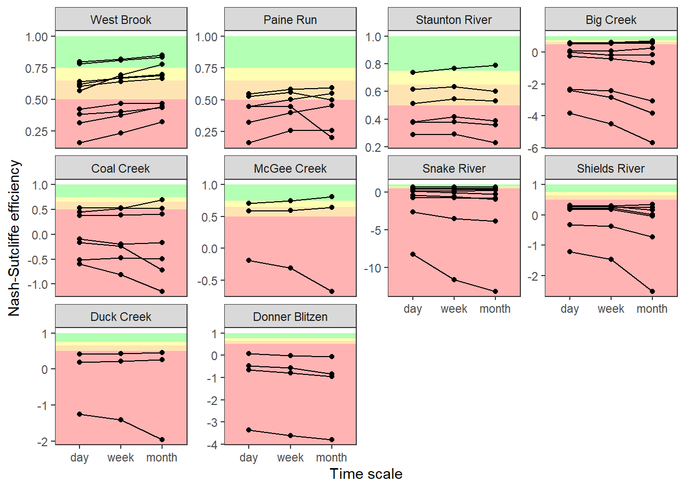
Generally, aggregating daily flow predictions to weekly or monthly means does not substantially change the accuracy of predicted data. However, there is a slight trend for accuracy (NSE) to increase with temporal aggregation for sites at which daily predictions are already fairly accurate. In contrast, for sites for which daily predictions are not accurate, temporal aggregation further decreases accuracy.