---
title: "Compare Population Outcomes"
---
```{r, include = FALSE, cache = FALSE}
library(tidyverse)
library(lubridate)
library(ggpubr)
library(egg)
library(RColorBrewer)
library(ggridges)
library(patchwork)
library(scales)
library(ggrepel)
source("Functions.R")
source("PlotResults.R")
source("ScenarioDefs.R")
```
**Purpose:** Compare emergent population outcomes across fixed habitat simulation runs.
## Setup
Load simulation results
```{r}
#| cache: false
## Null/cold only

# 95% cold
res           <- readRDS("results/TempOffset_ColdOnly_95percold.rds")
ibm_long_95null   <- res$ibm_long
habitat_df_95null <- res$habitat_df

# 75% cold
res           <- readRDS("results/TempOffset_ColdOnly_75percold.rds")
ibm_long_75null   <- res$ibm_long
habitat_df_75null <- res$habitat_df

# 50% cold
res           <- readRDS("results/TempOffset_ColdOnly_50percold.rds")
ibm_long_50null   <- res$ibm_long
habitat_df_50null <- res$habitat_df

# 25% cold
res           <- readRDS("results/TempOffset_ColdOnly_25percold.rds")
ibm_long_25null   <- res$ibm_long
habitat_df_25null <- res$habitat_df

# 5% cold
res           <- readRDS("results/TempOffset_ColdOnly_05percold.rds")
ibm_long_05null   <- res$ibm_long
habitat_df_05null <- res$habitat_df


## Cold + warm (same max pcmax)

# 95% cold / 5% warm
res           <- readRDS("results/TempOffset_ColdWarm_95percold.rds")
ibm_long_95   <- res$ibm_long
habitat_df_95 <- res$habitat_df

# 75% cold / 25% warm
res           <- readRDS("results/TempOffset_ColdWarm_75percold.rds")
ibm_long_75   <- res$ibm_long
habitat_df_75 <- res$habitat_df

# 50% cold / 50% warm
res           <- readRDS("results/TempOffset_ColdWarm_50percold.rds")
ibm_long_50   <- res$ibm_long
habitat_df_50 <- res$habitat_df

# 25% cold / 75% warm
res           <- readRDS("results/TempOffset_ColdWarm_25percold.rds")
ibm_long_25   <- res$ibm_long
habitat_df_25 <- res$habitat_df

# 5% cold / 95% warm
res           <- readRDS("results/TempOffset_ColdWarm_05percold.rds")
ibm_long_05   <- res$ibm_long
habitat_df_05 <- res$habitat_df


## Cold + warm (+0.1 max pcmax in warm)

# 95% cold / 5% warm
res           <- readRDS("results/TempOffset_ColdWarm_95percold_highPwarm.rds")
ibm_long_95_highpcm   <- res$ibm_long
habitat_df_95_highpcm <- res$habitat_df

# 75% cold / 25% warm
res           <- readRDS("results/TempOffset_ColdWarm_75percold_highPwarm.rds")
ibm_long_75_highpcm   <- res$ibm_long
habitat_df_75_highpcm <- res$habitat_df

# 50% cold / 50% warm
res           <- readRDS("results/TempOffset_ColdWarm_50percold_highPwarm.rds")
ibm_long_50_highpcm   <- res$ibm_long
habitat_df_50_highpcm <- res$habitat_df

# 25% cold / 75% warm
res           <- readRDS("results/TempOffset_ColdWarm_25percold_highPwarm.rds")
ibm_long_25_highpcm   <- res$ibm_long
habitat_df_25_highpcm <- res$habitat_df

# 5% cold / 95% warm
res           <- readRDS("results/TempOffset_ColdWarm_05percold_highPwarm.rds")
ibm_long_05_highpcm   <- res$ibm_long
habitat_df_05_highpcm <- res$habitat_df


sim_params    <- res$params
exp_start_date <- sim_params$mindate + years(sim_params$nyears_burnin)

rm(res)
```
Summarize within each scenario before combining to avoid loading all five full data frames into memory simultaneously. The Oct 1 census data (1 row per fish per year) and the patch-level growth totals (1 row per year × patch) are the only data structures that need to be combined across scenarios.
```{r}
#| cache: false
# ── Scenario metadata ─────────────────────────────────────────────────────────
scen_meta <- tibble(
  scen_key  = c("95", "75", "50", "25", "05"),
  label     = c("95% cold", "75% cold", "50% cold", "25% cold", "5% cold"),
  prop_cold = c(0.95, 0.75, 0.50, 0.25, 0.05)
)

scen_pal <- setNames(
  hcl.colors(5, "Zissou 1"),
  scen_meta$label
)


# Linetype and shape palettes for habitat availability
hab_cols  <- c("Cold only" = "#6BAED6",  "Cold + Warm" = "#FC8D59",   "Cold + Warm (high P)" = "#B30000")
hab_lty   <- c("Cold only" = "solid" ,   "Cold + Warm" = "solid",     "Cold + Warm (high P)" = "solid")
hab_shape <- c("Cold only" = 16,         "Cold + Warm" = 16,          "Cold + Warm (high P)" = 16)

# Helper: extract Oct 1 experimental-period rows from one ibm_long
# Filtering before bind_rows() keeps only ~1/365th of each data frame.
extract_oct1_exp <- function(ibm_long, scen_key) {
  ibm_long |>
    filter(date >= exp_start_date,
           month(date) == 10, day(date) == 1,
           survived == 1) |>
    mutate(scen_key  = scen_key,
           year      = year(date),
           age_class = floor(age))
}

# Helper: compute per-year biomass accrual by patch (experimental period only).
# Summarises to n_years × 2 rows per scenario before combining.
compute_patch_growth <- function(ibm_long, scen_key) {
  ibm_long |>
    filter(date >= exp_start_date, !is.na(ggd)) |>
    mutate(daily_growth_g = weight * ggd, year = year(date)) |>
    group_by(year, patch) |>
    summarise(total_g = sum(daily_growth_g, na.rm = TRUE), .groups = "drop") |>
    mutate(scen_key = scen_key)
}

# ── Oct 1 census: experimental period, both hab types, all scenarios ──────────
exp_oct1 <- bind_rows(
  bind_rows(
    extract_oct1_exp(ibm_long_95, "95"),
    extract_oct1_exp(ibm_long_75, "75"),
    extract_oct1_exp(ibm_long_50, "50"),
    extract_oct1_exp(ibm_long_25, "25"),
    extract_oct1_exp(ibm_long_05, "05")
  ) |> mutate(hab_type = "Cold + Warm"),
  bind_rows(
    extract_oct1_exp(ibm_long_95_highpcm, "95"),
    extract_oct1_exp(ibm_long_75_highpcm, "75"),
    extract_oct1_exp(ibm_long_50_highpcm, "50"),
    extract_oct1_exp(ibm_long_25_highpcm, "25"),
    extract_oct1_exp(ibm_long_05_highpcm, "05")
  ) |> mutate(hab_type = "Cold + Warm (high P)"),
  bind_rows(
    extract_oct1_exp(ibm_long_95null, "95"),
    extract_oct1_exp(ibm_long_75null, "75"),
    extract_oct1_exp(ibm_long_50null, "50"),
    extract_oct1_exp(ibm_long_25null, "25"),
    extract_oct1_exp(ibm_long_05null, "05")
  ) |> mutate(hab_type = "Cold only")
) |>
  left_join(scen_meta, by = "scen_key") |>
  mutate(
    label    = factor(label,    levels = scen_meta$label),
    hab_type = factor(hab_type, levels = c("Cold only", "Cold + Warm", "Cold + Warm (high P)"))
  )

# ── Annual biomass accrual by patch, both hab types, all scenarios ────────────
patch_growth <- bind_rows(
  bind_rows(
    compute_patch_growth(ibm_long_95, "95"),
    compute_patch_growth(ibm_long_75, "75"),
    compute_patch_growth(ibm_long_50, "50"),
    compute_patch_growth(ibm_long_25, "25"),
    compute_patch_growth(ibm_long_05, "05")
  ) |> mutate(hab_type = "Cold + Warm"),
  bind_rows(
    compute_patch_growth(ibm_long_95_highpcm, "95"),
    compute_patch_growth(ibm_long_75_highpcm, "75"),
    compute_patch_growth(ibm_long_50_highpcm, "50"),
    compute_patch_growth(ibm_long_25_highpcm, "25"),
    compute_patch_growth(ibm_long_05_highpcm, "05")
  ) |> mutate(hab_type = "Cold + Warm (high P)"),
  bind_rows(
    compute_patch_growth(ibm_long_95null, "95"),
    compute_patch_growth(ibm_long_75null, "75"),
    compute_patch_growth(ibm_long_50null, "50"),
    compute_patch_growth(ibm_long_25null, "25"),
    compute_patch_growth(ibm_long_05null, "05")
  ) |> mutate(hab_type = "Cold only")
) |>
  left_join(scen_meta, by = "scen_key") |>
  mutate(
    label    = factor(label,    levels = scen_meta$label),
    hab_type = factor(hab_type, levels = c("Cold only", "Cold + Warm", "Cold + Warm (high P)"))
  )

# ── Annual population totals per scenario × hab_type × year ──────────────────
exp_pop_yr <- exp_oct1 |>
  group_by(hab_type, label, prop_cold, year) |>
  summarise(n = n(), biomass_kg = sum(weight) / 1000, .groups = "drop")
```
## Abundance and biomass
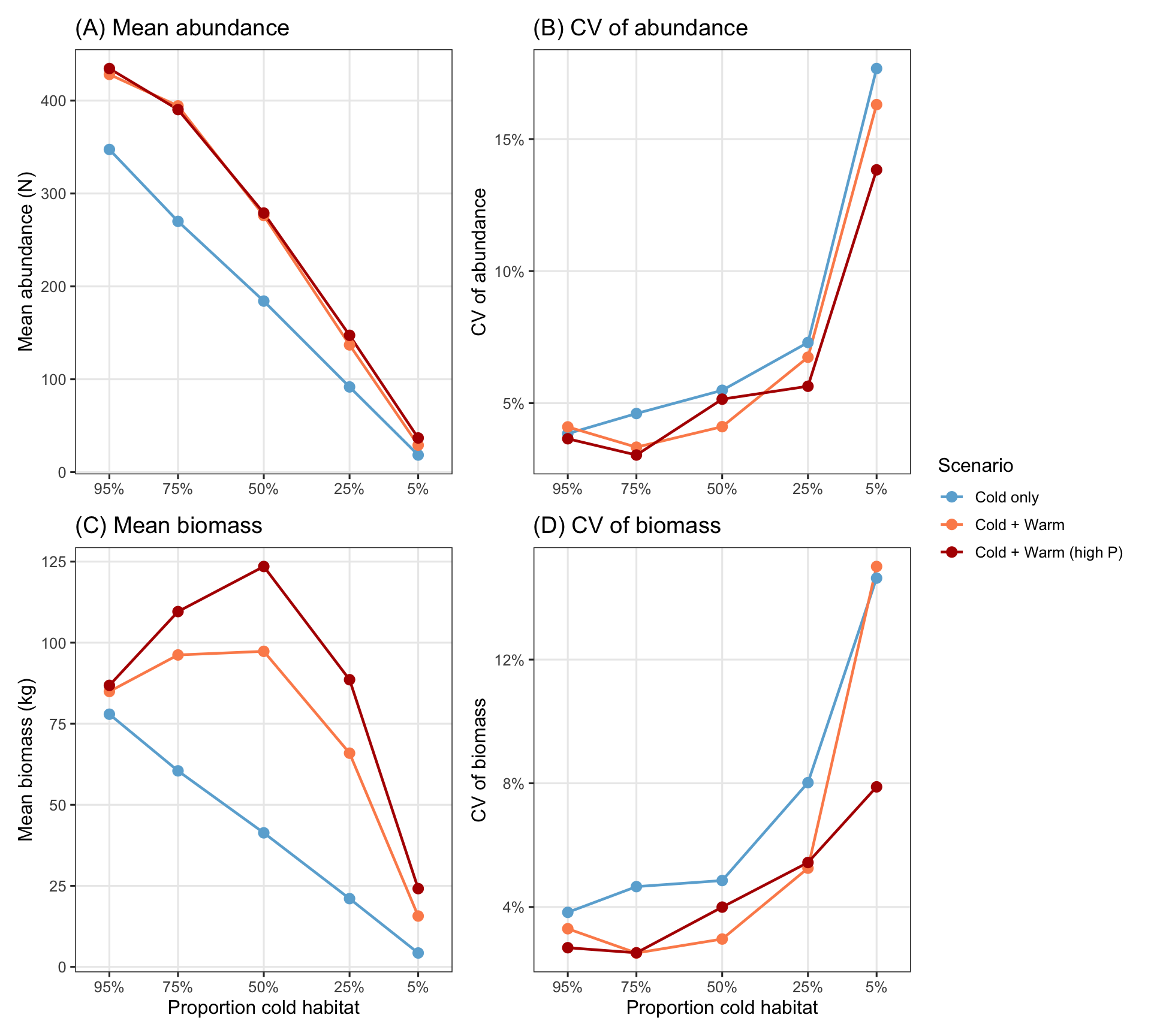
Mean and coefficient of variation (CV) of Oct 1 abundance and biomass during the experimental period, as a function of the proportion of cold habitat.
```{r}
#| fig-width: 10
#| fig-height: 9
pop_sum <- exp_pop_yr |>
  group_by(hab_type, label, prop_cold) |>
  summarise(
    mean_n  = mean(n),
    cv_n    = sd(n) / mean(n),
    mean_b  = mean(biomass_kg),
    cv_b    = sd(biomass_kg) / mean(biomass_kg),
    .groups = "drop"
  )

write_csv(pop_sum, "pop_sum.csv")

cold_x <- function(xlab = NULL) {
  list(
    scale_x_continuous(
      breaks = scen_meta$prop_cold,
      labels = scales::label_percent(accuracy = 1),
      limits = c(0, 1),
      transform = "reverse"
    ),
    labs(x = xlab)
  )
}

# Shared scale additions for hab_type encoding (linetype + shape merged legend)
hab_scales <- list(
  scale_linetype_manual(values = hab_lty,   name = "Habitat"),
  scale_shape_manual(  values = hab_shape,  name = "Habitat")
)

ab_plot <- function(data, y_var, y_lab, title_str, pct_y = FALSE) {
  p <- ggplot(data, aes(x = prop_cold, y = .data[[y_var]], color = hab_type)) +
    geom_line(aes(linetype = hab_type, group = hab_type), linetype = "solid", linewidth = 0.8) +
    geom_point(aes(shape = hab_type), size = 3, shape = 16) +
    scale_color_manual(values = hab_cols, name = "Scenario") +
    # hab_scales +
    labs(y = y_lab, title = title_str) +
    theme_bw(base_size = 12) +
    theme(panel.grid.minor = element_blank())
  if (pct_y) p <- p + scale_y_continuous(labels = scales::label_percent(accuracy = 1))
  p
}

p_mean_n <- ab_plot(pop_sum, "mean_n", "Mean abundance (N)",  "(A) Mean abundance")       + cold_x()
p_cv_n   <- ab_plot(pop_sum, "cv_n",   "CV of abundance",     "(B) CV of abundance", TRUE) + cold_x()
p_mean_b <- ab_plot(pop_sum, "mean_b", "Mean biomass (kg)",   "(C) Mean biomass")          + cold_x("Proportion cold habitat")
p_cv_b   <- ab_plot(pop_sum, "cv_b",   "CV of biomass",       "(D) CV of biomass",   TRUE) + cold_x("Proportion cold habitat")

(p_mean_n + p_cv_n) / (p_mean_b + p_cv_b) +
  plot_layout(guides = "collect") &
  theme(legend.position = "right")
```
```{r}
#| fig-width: 9.5
#| fig-height: 4
#|
p_rd_n <- pop_sum %>%
  select(hab_type, label, prop_cold, mean_n) %>%
  pivot_wider(names_from = hab_type, values_from = mean_n) %>%
  rename("cold_only" = "Cold only", "cold_warm" = "Cold + Warm",  "high_P" = "Cold + Warm (high P)") %>%
  mutate(rd_coldwarm = (cold_warm - cold_only)/cold_only,
         rd_highp = (high_P - cold_only)/cold_only) %>%
  pivot_longer(rd_coldwarm:rd_highp, names_to = "hab_type", values_to = "reldiff") %>%
  mutate(hab_type = recode(hab_type, "rd_coldwarm" = "Cold + Warm", "rd_highp" = "Cold + Warm (high P)")) %>%
  ggplot(aes(x = prop_cold, y = reldiff, color = hab_type)) +
  geom_line(aes(linetype = hab_type, group = hab_type), linetype = "solid", linewidth = 0.8) +
  geom_point(aes(shape = hab_type), size = 3, shape = 16) +
  scale_color_manual(values = hab_cols, name = "Scenario") +
  labs(y = "Relative difference in abundance") +
  theme_bw(base_size = 12) +
  theme(panel.grid.minor = element_blank()) +
  cold_x("Proportion cold habitat") +
  scale_y_continuous(labels = scales::label_percent(accuracy = 1), limits = c(0,5))

p_rd_b <- pop_sum %>%
  select(hab_type, label, prop_cold, mean_b) %>%
  pivot_wider(names_from = hab_type, values_from = mean_b) %>%
  rename("cold_only" = "Cold only", "cold_warm" = "Cold + Warm",  "high_P" = "Cold + Warm (high P)") %>%
  mutate(rd_coldwarm = (cold_warm - cold_only)/cold_only,
         rd_highp = (high_P - cold_only)/cold_only) %>%
  pivot_longer(rd_coldwarm:rd_highp, names_to = "hab_type", values_to = "reldiff") %>%
  mutate(hab_type = recode(hab_type, "rd_coldwarm" = "Cold + Warm", "rd_highp" = "Cold + Warm (high P)")) %>%
  ggplot(aes(x = prop_cold, y = reldiff, color = hab_type)) +
  geom_line(aes(linetype = hab_type, group = hab_type), linetype = "solid", linewidth = 0.8) +
  geom_point(aes(shape = hab_type), size = 3, shape = 16) +
  scale_color_manual(values = hab_cols, name = "Scenario") +
  labs(y = "Relative difference in biomass") +
  theme_bw(base_size = 12) +
  theme(panel.grid.minor = element_blank()) +
  cold_x("Proportion cold habitat") +
  scale_y_continuous(labels = scales::label_percent(accuracy = 1), limits = c(0,5))


p_rd_n + p_rd_b +
  plot_layout(guides = "collect") &
  theme(legend.position = "right", plot.title = element_text(size = 15), plot.subtitle = element_text(face = "italic")) &
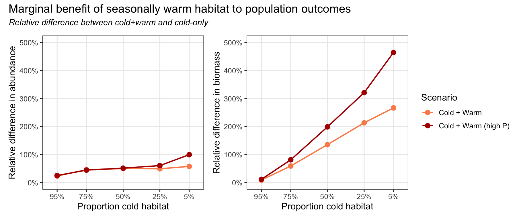
  plot_annotation(title = "Marginal benefit of seasonally warm habitat to population outcomes",
                  subtitle = "Relative difference between cold+warm and cold-only")
```
## Weight-at-age
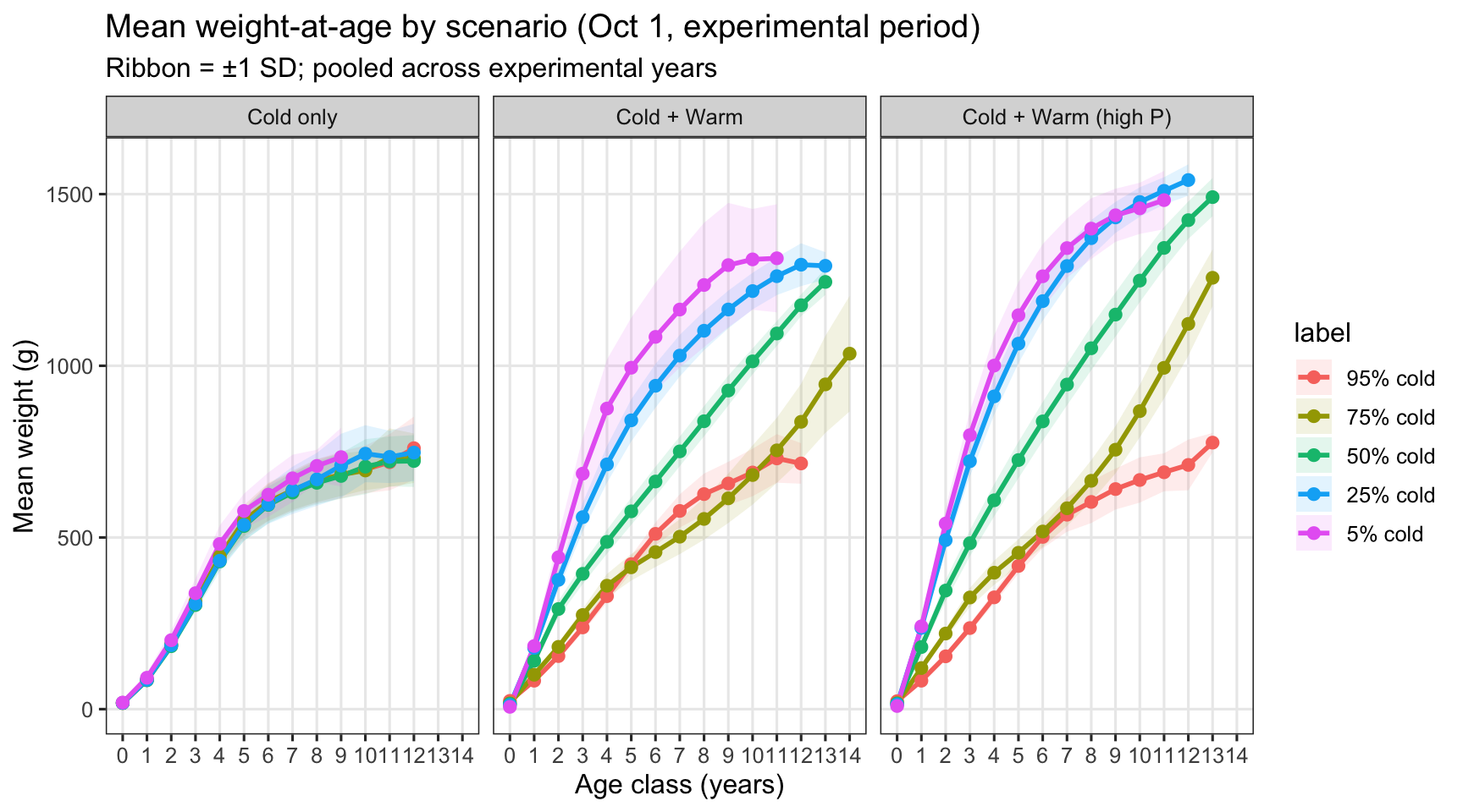
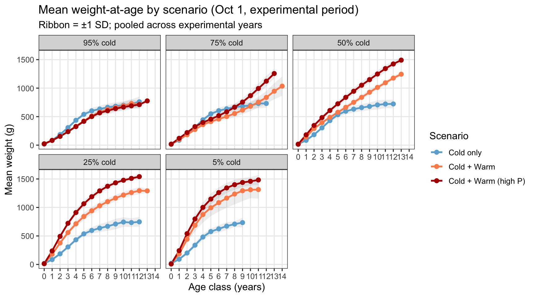
Mean weight at each integer age class, pooled across all Oct 1 experimental-period censuses, compared across scenarios. Lines colored from blue (cold-dominant) to red/orange (warm-dominant).
```{r}
#| fig-width: 9
#| fig-height: 5
waa_scen <- exp_oct1 |>
  group_by(hab_type, label, prop_cold, age_class) |>
  summarise(
    mean_wt = mean(weight),
    sd_wt   = sd(weight),
    n       = n(),
    .groups = "drop"
  ) |>
  filter(n >= 5)

age_breaks_scen <- sort(unique(waa_scen$age_class))


ggplot(waa_scen, aes(x = age_class, y = mean_wt,
                      color = label, fill = label,
                      group = interaction(label, hab_type))) +
  geom_ribbon(aes(ymin = pmax(0, mean_wt - sd_wt), ymax = mean_wt + sd_wt),
              alpha = 0.12, color = NA) +
  geom_line(linewidth = 1, linetype = "solid") +
  geom_point(aes(shape = hab_type), size = 2.5, shape = 16) +
  # scale_color_manual(values = hab_cols, name = "Scenario") +
  # scale_fill_manual(values  = hab_cols, name = "Scenario") +
  # scale_linetype_manual(values = hab_lty,   name = "Habitat") +
  # scale_shape_manual(  values = hab_shape,  name = "Habitat") +
  scale_x_continuous(breaks = age_breaks_scen) +
  labs(
    x = "Age class (years)", y = "Mean weight (g)",
    title = "Mean weight-at-age by scenario (Oct 1, experimental period)",
    subtitle = "Ribbon = \u00b11 SD; pooled across experimental years"
  ) +
  theme_bw(base_size = 12) +
  theme(legend.position = "right", panel.grid.minor = element_blank()) +
  facet_wrap(~label) +
  facet_wrap(~hab_type)
ggplot(waa_scen, aes(x = age_class, y = mean_wt,
                      color = hab_type, fill = label,
                      group = interaction(label, hab_type))) +
  geom_ribbon(aes(ymin = pmax(0, mean_wt - sd_wt), ymax = mean_wt + sd_wt),
              alpha = 0.12, color = NA) +
  geom_line(linewidth = 1, linetype = "solid") +
  geom_point(aes(shape = hab_type), size = 2.5, shape = 16) +
  scale_color_manual(values = hab_cols, name = "Scenario") +
  scale_fill_manual(values  = hab_cols, name = "Scenario") +
  # scale_linetype_manual(values = hab_lty,   name = "Habitat") +
  # scale_shape_manual(  values = hab_shape,  name = "Habitat") +
  scale_x_continuous(breaks = age_breaks_scen) +
  labs(
    x = "Age class (years)", y = "Mean weight (g)",
    title = "Mean weight-at-age by scenario (Oct 1, experimental period)",
    subtitle = "Ribbon = \u00b11 SD; pooled across experimental years"
  ) +
  theme_bw(base_size = 12) +
  theme(legend.position = "right", panel.grid.minor = element_blank()) +
  facet_wrap(~label)
```
## Age structure
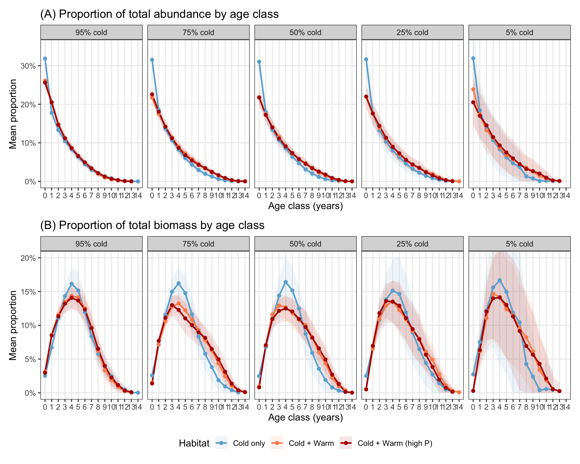
Mean proportion of total abundance and biomass at each age class during the experimental period, compared across scenarios.
```{r}
#| fig-width: 10
#| fig-height: 8
# Per-year counts and biomass by age class (fill zeros for absent classes)
age_yr_scen <- exp_oct1 |>
  group_by(hab_type, label, prop_cold, year, age_class) |>
  summarise(n = n(), biomass_kg = sum(weight) / 1000, .groups = "drop") |>
  complete(nesting(hab_type, label, prop_cold), year, age_class,
           fill = list(n = 0, biomass_kg = 0))

# Proportional abundance by age class
prop_n_scen <- age_yr_scen |>
  group_by(hab_type, label, prop_cold, year) |>
  mutate(prop = n / sum(n)) |>
  ungroup() |>
  group_by(hab_type, label, prop_cold, age_class) |>
  summarise(mean_prop = mean(prop), sd_prop = sd(prop), .groups = "drop") |>
  filter(mean_prop > 0)

# Proportional biomass by age class
prop_b_scen <- age_yr_scen |>
  group_by(hab_type, label, prop_cold, year) |>
  mutate(prop = biomass_kg / sum(biomass_kg)) |>
  ungroup() |>
  group_by(hab_type, label, prop_cold, age_class) |>
  summarise(mean_prop = mean(prop), sd_prop = sd(prop), .groups = "drop") |>
  filter(mean_prop > 0)

age_breaks_struct <- sort(unique(c(prop_n_scen$age_class, prop_b_scen$age_class)))

age_struct_plot <- function(data, title_str) {
  ggplot(data, aes(x = age_class, y = mean_prop,
                   color = hab_type, fill = hab_type,
                   # linetype = hab_type,
                   group = interaction(label, hab_type))) +
    geom_ribbon(
      aes(ymin = pmax(0, mean_prop - sd_prop), ymax = mean_prop + sd_prop),
      alpha = 0.10, color = NA
    ) +
    geom_line(linewidth = 0.9) +
    geom_point(size = 2, shape = 16) +
    scale_color_manual(values = hab_cols, name = "Habitat") +
    scale_fill_manual(values  = hab_cols, name = "Habitat") +
    # scale_linetype_manual(values = hab_lty,   name = "Habitat") +
    # scale_shape_manual(  values = hab_shape,  name = "Habitat") +
    scale_x_continuous(breaks = age_breaks_struct) +
    scale_y_continuous(labels = scales::label_percent(accuracy = 1)) +
    labs(x = "Age class (years)", y = "Mean proportion", title = title_str) +
    theme_bw(base_size = 12) +
    theme(panel.grid.minor = element_blank(), legend.position = "bottom") +
    facet_wrap(~label, nrow = 1)
}

p_prop_n <- age_struct_plot(prop_n_scen,
                             "(A) Proportion of total abundance by age class") + coord_cartesian(ylim = c(0,0.35))
p_prop_b <- age_struct_plot(prop_b_scen,
                             "(B) Proportion of total biomass by age class") + coord_cartesian(ylim = c(0,0.2))

p_prop_n / p_prop_b + plot_layout(guides = "collect") & theme(legend.position = "bottom")
```
## Warm habitat contribution
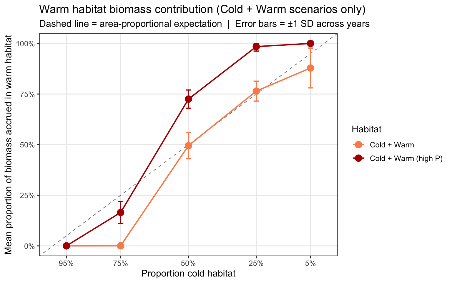
Mean (± SD across experimental years) proportion of annual population-level biomass accrued in warm habitat, as a function of cold vs. warm habitat availability. Biomass accrual computed across all strategies as the sum of daily growth (weight × ggd) in each patch.
```{r}
#| fig-width: 8
#| fig-height: 5
# Cold-only (null) scenarios have no warm patch, so their warm contribution is
# 0 by definition and is not shown here.
warm_share_scen <- patch_growth |>
  filter(hab_type %in% c("Cold + Warm", "Cold + Warm (high P)")) |>
  pivot_wider(names_from = patch, values_from = total_g, values_fill = 0) |>
  mutate(
    pos_warm   = pmax(warm, 0),
    pos_cold   = pmax(cold, 0),
    f_warm_pos = if_else(pos_warm + pos_cold > 0,
                         pos_warm / (pos_warm + pos_cold),
                         NA_real_)
  ) |>
  group_by(hab_type, label, prop_cold) |>
  summarise(
    mean_f_warm = mean(f_warm_pos, na.rm = TRUE),
    sd_f_warm   = sd(f_warm_pos,   na.rm = TRUE),
    .groups     = "drop"
  )

ggplot(warm_share_scen, aes(x = prop_cold, y = mean_f_warm, color = hab_type, group = hab_type)) +
  # Area-proportional expectation: f_warm = 1 - prop_cold
  geom_abline(slope = 1, intercept = 1, linetype = "dashed",
              color = "grey50", linewidth = 0.4) +
  geom_errorbar(
    aes(ymin = pmax(0, mean_f_warm - sd_f_warm),
        ymax = pmin(1, mean_f_warm + sd_f_warm)),
    width = 0.02, linewidth = 0.7
  ) +
  geom_line(linewidth = 0.8) +
  geom_point(size = 4, shape = 16) +
  # scale_shape_manual(  values = hab_shape,  name = "Habitat") +
  scale_color_manual(values = hab_cols, name = "Habitat") +
  scale_x_continuous(
    breaks = scen_meta$prop_cold,
    labels = scales::label_percent(accuracy = 1),
    limits = c(0, 1),
    transform = "reverse"
  ) +
  scale_y_continuous(labels = scales::label_percent(accuracy = 1),
                     limits = c(0, 1)) +
  labs(
    x        = "Proportion cold habitat",
    y        = "Mean proportion of biomass accrued in warm habitat",
    title    = "Warm habitat biomass contribution (Cold + Warm scenarios only)",
    subtitle = "Dashed line = area-proportional expectation  |  Error bars = \u00b11 SD across years"
  ) +
  theme_bw(base_size = 12) +
  theme(panel.grid.minor = element_blank(), legend.position = "right")
```
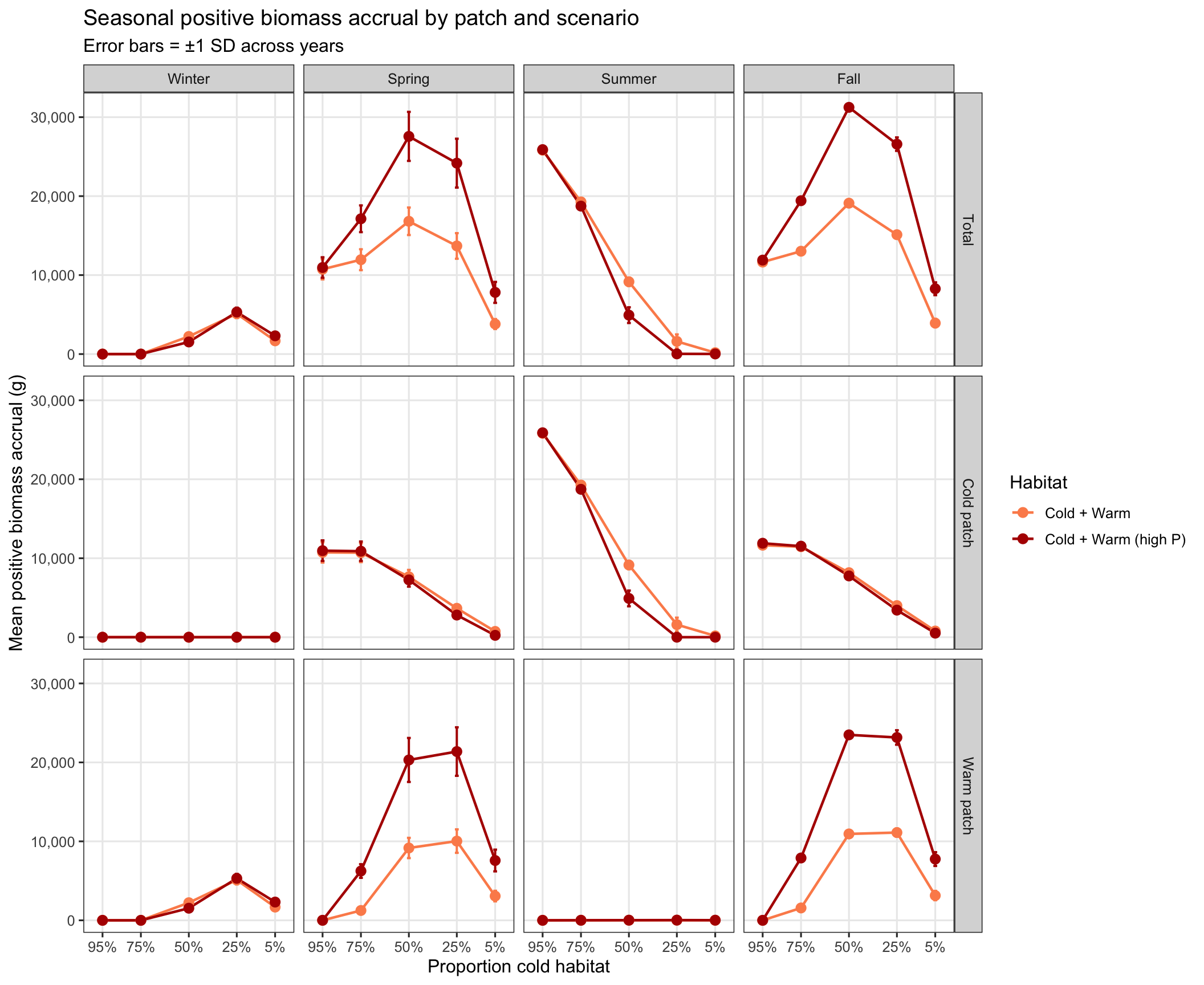
Mean positive biomass accrual per season, broken down by patch (total, cold, warm), showing absolute growth magnitude across cold habitat availability scenarios.
```{r}
#| fig-width: 11
#| fig-height: 9
compute_patch_growth_seasonal <- function(ibm_long, scen_key) {
  ibm_long |>
    filter(date >= exp_start_date, !is.na(ggd)) |>
    mutate(
      daily_growth_g = weight * ggd,
      year   = year(date),
      month  = month(date),
      season = case_when(
        month %in% c(12, 1, 2)  ~ "Winter",
        month %in% c(3, 4, 5)   ~ "Spring",
        month %in% c(6, 7, 8)   ~ "Summer",
        month %in% c(9, 10, 11) ~ "Fall"
      ),
      season = factor(season, levels = c("Winter", "Spring", "Summer", "Fall"))
    ) |>
    group_by(year, season, patch) |>
    summarise(total_g = sum(daily_growth_g, na.rm = TRUE), .groups = "drop") |>
    mutate(scen_key = scen_key)
}

patch_growth_seasonal <- bind_rows(
  bind_rows(
    compute_patch_growth_seasonal(ibm_long_95, "95"),
    compute_patch_growth_seasonal(ibm_long_75, "75"),
    compute_patch_growth_seasonal(ibm_long_50, "50"),
    compute_patch_growth_seasonal(ibm_long_25, "25"),
    compute_patch_growth_seasonal(ibm_long_05, "05")
  ) |> mutate(hab_type = "Cold + Warm"),
  bind_rows(
    compute_patch_growth_seasonal(ibm_long_95_highpcm, "95"),
    compute_patch_growth_seasonal(ibm_long_75_highpcm, "75"),
    compute_patch_growth_seasonal(ibm_long_50_highpcm, "50"),
    compute_patch_growth_seasonal(ibm_long_25_highpcm, "25"),
    compute_patch_growth_seasonal(ibm_long_05_highpcm, "05")
  ) |> mutate(hab_type = "Cold + Warm (high P)")
) |>
  left_join(scen_meta, by = "scen_key") |>
  mutate(
    label    = factor(label,    levels = scen_meta$label),
    hab_type = factor(hab_type, levels = c("Cold + Warm", "Cold + Warm (high P)", "Cold only"))
  )

per_patch <- patch_growth_seasonal |>
  filter(hab_type %in% c("Cold + Warm", "Cold + Warm (high P)")) |>
  mutate(pos_g = pmax(total_g, 0)) |>
  select(hab_type, year, season, patch, pos_g, label, prop_cold)

season_raw <- bind_rows(
  per_patch |>
    group_by(hab_type, year, season, label, prop_cold) |>
    summarise(pos_g = sum(pos_g, na.rm = TRUE), .groups = "drop") |>
    mutate(patch_label = "Total"),
  per_patch |> mutate(patch_label = case_when(
    patch == "cold" ~ "Cold patch",
    patch == "warm" ~ "Warm patch"
  ))
) |>
  mutate(patch_label = factor(patch_label,
                              levels = c("Total", "Cold patch", "Warm patch"))) |>
  group_by(hab_type, label, prop_cold, season, patch_label) |>
  summarise(
    mean_pos_g = mean(pos_g, na.rm = TRUE),
    sd_pos_g   = sd(pos_g,   na.rm = TRUE),
    .groups = "drop"
  )

ggplot(season_raw, aes(x = prop_cold, y = mean_pos_g, color = hab_type, group = hab_type)) +
  geom_errorbar(
    aes(ymin = pmax(0, mean_pos_g - sd_pos_g),
        ymax = mean_pos_g + sd_pos_g),
    width = 0.02, linewidth = 0.7
  ) +
  geom_line(linewidth = 0.8) +
  geom_point(size = 3, shape = 16) +
  # scale_shape_manual(values = hab_shape,  name = "Habitat") +
  scale_color_manual(values = hab_cols, name = "Habitat") +
  scale_x_continuous(
    breaks = scen_meta$prop_cold,
    labels = scales::label_percent(accuracy = 1),
    limits = c(0, 1),
    transform = "reverse"
  ) +
  scale_y_continuous(labels = scales::label_comma()) +
  facet_grid(patch_label ~ season) +
  labs(
    x        = "Proportion cold habitat",
    y        = "Mean positive biomass accrual (g)",
    title    = "Seasonal positive biomass accrual by patch and scenario",
    subtitle = "Error bars = \u00b11 SD across years"
  ) +
  theme_bw(base_size = 12) +
  theme(panel.grid.minor = element_blank(), legend.position = "right")
```
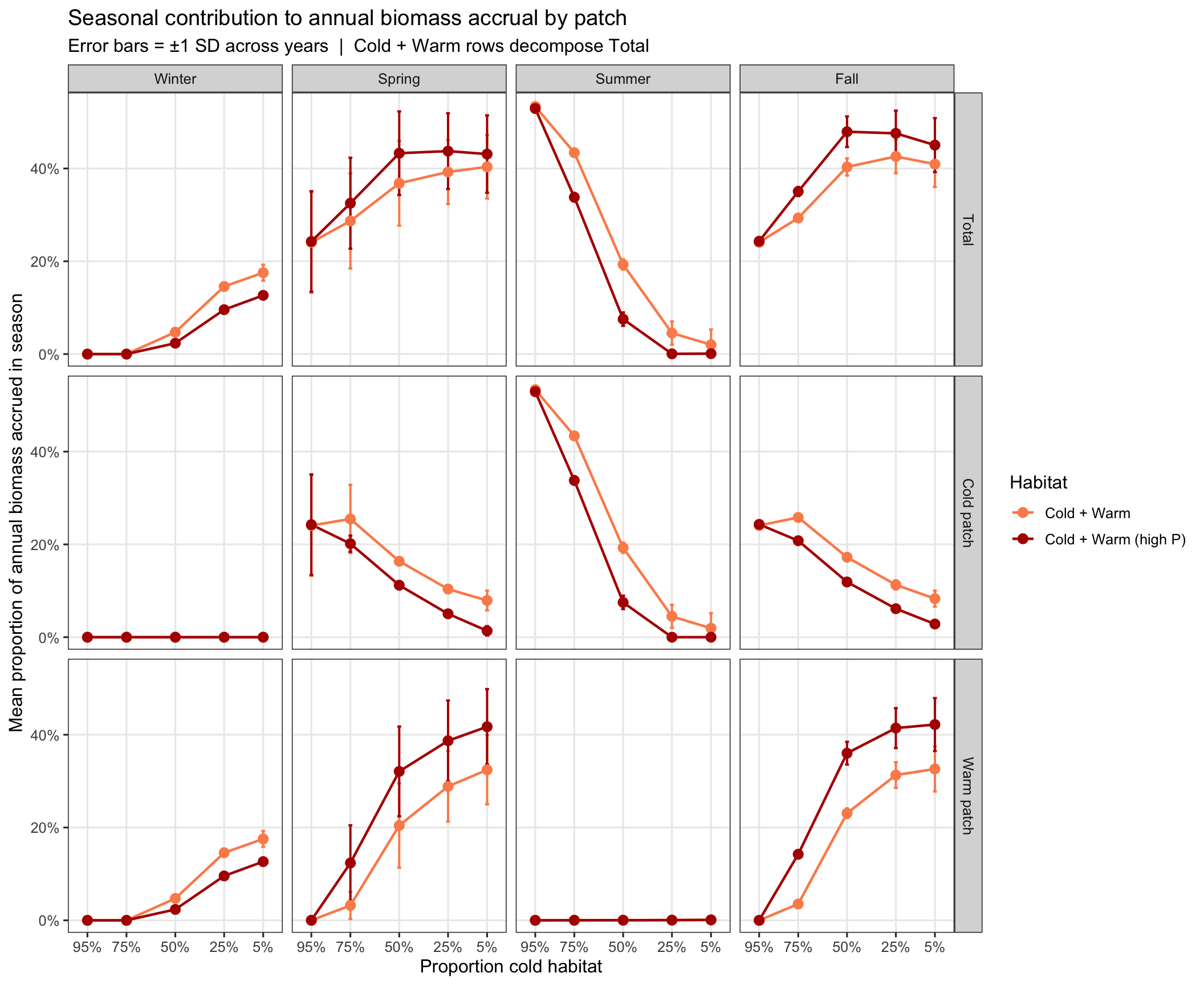
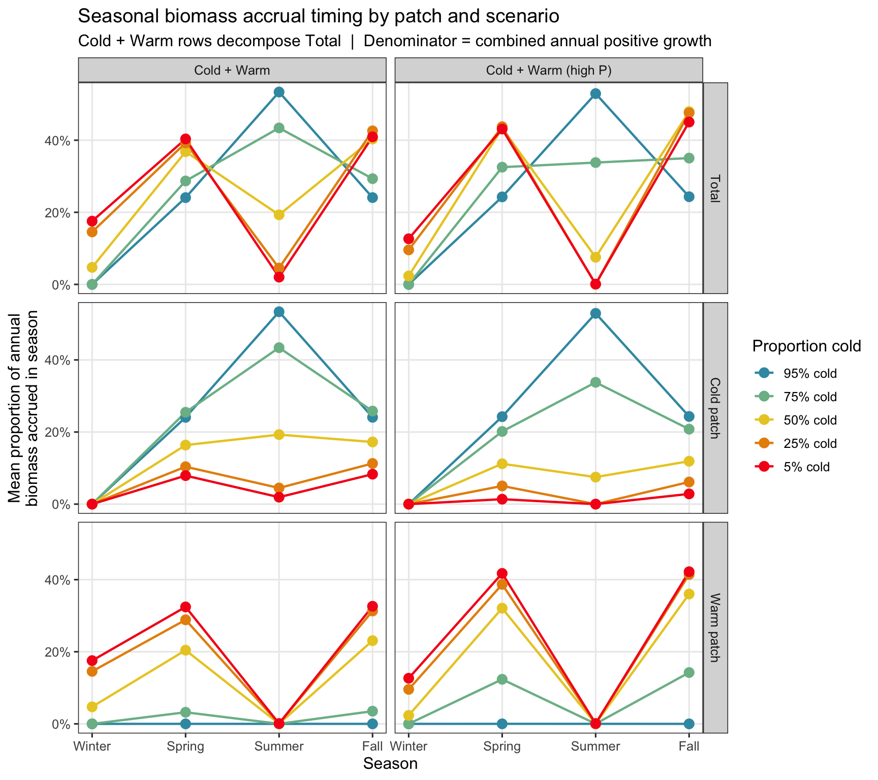
Each season's positive biomass accrual as a proportion of total annual positive growth (both patches combined), broken down by patch. The denominator is always the combined annual total, so the cold and warm patch rows decompose the total row and together sum to 100%.
```{r}
#| fig-width: 11
#| fig-height: 9
# Annual total positive growth (both patches, all seasons) — the shared denominator
annual_total <- patch_growth_seasonal |>
  filter(hab_type %in% c("Cold + Warm", "Cold + Warm (high P)")) |>
  mutate(pos_g = pmax(total_g, 0)) |>
  group_by(hab_type, year, label, prop_cold) |>
  summarise(annual_pos_g = sum(pos_g, na.rm = TRUE), .groups = "drop")

per_patch_season <- patch_growth_seasonal |>
  filter(hab_type %in% c("Cold + Warm", "Cold + Warm (high P)")) |>
  mutate(pos_g = pmax(total_g, 0)) |>
  select(hab_type, year, season, patch, pos_g, label, prop_cold)

season_share_patch <- bind_rows(
  per_patch_season |>
    group_by(hab_type, year, season, label, prop_cold) |>
    summarise(pos_g = sum(pos_g, na.rm = TRUE), .groups = "drop") |>
    mutate(patch_label = "Total"),
  per_patch_season |>
    filter(patch == "cold") |>
    mutate(patch_label = "Cold patch") |>
    select(-patch),
  per_patch_season |>
    filter(patch == "warm") |>
    mutate(patch_label = "Warm patch") |>
    select(-patch)
) |>
  left_join(annual_total, by = c("hab_type", "year", "label", "prop_cold")) |>
  mutate(
    patch_label = factor(patch_label,
                         levels = c("Total", "Cold patch", "Warm patch")),
    f_season    = if_else(annual_pos_g > 0, pos_g / annual_pos_g, NA_real_)
  ) |>
  group_by(hab_type, label, prop_cold, season, patch_label) |>
  summarise(
    mean_f_season = mean(f_season, na.rm = TRUE),
    sd_f_season   = sd(f_season,   na.rm = TRUE),
    .groups = "drop"
  )

# Faceted by season (columns) × patch (rows); prop_cold on x-axis
ggplot(season_share_patch, aes(x = prop_cold, y = mean_f_season, color = hab_type, group = hab_type)) +
  geom_errorbar(
    aes(ymin = pmax(0, mean_f_season - sd_f_season),
        ymax = pmin(1, mean_f_season + sd_f_season)),
    width = 0.02, linewidth = 0.7
  ) +
  geom_line(linewidth = 0.8) +
  geom_point(size = 3, shape = 16) +
  # scale_shape_manual(values = hab_shape,  name = "Habitat") +
  scale_color_manual(values = hab_cols, name = "Habitat") +
  scale_x_continuous(
    breaks = scen_meta$prop_cold,
    labels = scales::label_percent(accuracy = 1),
    limits = c(0, 1),
    transform = "reverse"
  ) +
  scale_y_continuous(labels = scales::label_percent(accuracy = 1)) +
  facet_grid(patch_label ~ season) +
  labs(
    x        = "Proportion cold habitat",
    y        = "Mean proportion of annual biomass accrued in season",
    title    = "Seasonal contribution to annual biomass accrual by patch",
    subtitle = "Error bars = \u00b11 SD across years  |  Cold + Warm rows decompose Total"
  ) +
  theme_bw(base_size = 12) +
  theme(panel.grid.minor = element_blank(), legend.position = "right")
```
```{r}
#| fig-width: 9
#| fig-height: 8
# Season on x-axis, colored by scenario, patch in rows
ggplot(season_share_patch,
       aes(x = as.numeric(season), y = mean_f_season,
           color = label, group = label)) +
  geom_line(linewidth = 0.8) +
  geom_point(size = 3) +
  scale_color_manual(values = scen_pal, name = "Proportion cold") +
  scale_x_continuous(
    breaks = 1:4,
    labels = levels(season_share_patch$season)
  ) +
  scale_y_continuous(labels = scales::label_percent(accuracy = 1)) +
  facet_grid(patch_label ~ hab_type) +
  labs(
    x        = "Season",
    y        = "Mean proportion of annual\nbiomass accrued in season",
    title    = "Seasonal biomass accrual timing by patch and scenario",
    subtitle = "Cold + Warm rows decompose Total  |  Denominator = combined annual positive growth"
  ) +
  theme_bw(base_size = 12) +
  theme(panel.grid.minor = element_blank(), legend.position = "right")
```
**As we lose cold-water habitat and gain warm-water habitat, the growth regime becomes increasingly bi-modal; with an increasing share of annual biomass being accrued in the warm patch in the non-summer seasons (particularly spring and autumn), and a decreasing share of annual biomass being accrued in summer in the cold patch. Moreover, the relative importance of warm habitat to spring and fall biomass accrual increases when maximum consumption rates (P-values) are greater in the warm habitat.**