---
title: "Mechanistic Drivers"
---
```{r, include = FALSE, cache = FALSE}
library(tidyverse)
library(lubridate)
library(ggpubr)
library(egg)
library(RColorBrewer)
library(ggridges)
library(patchwork)
library(scales)
library(ggrepel)
source("Functions.R")
source("PlotResults.R")
source("ScenarioDefs.R")
```
**Purpose:** Describe mechanistic drivers of differences in abundance and biomass across simulations.
## Setup
Load each result .rds object and bind directly into a list. Using a helper function ensures each `res` object is freed from memory as soon as `ibm_long` is extracted, avoiding duplicate references that would force R to copy the data frames.
```{r}
#| cache: false
# Extract params from one file (small object)
res            <- readRDS("results/TempOffset_ColdWarm_05percold_highPwarm.rds")
sim_params     <- res$params
exp_start_date <- sim_params$mindate + years(sim_params$nyears_burnin)
rm(res)

# Helper: read one scenario, extract ibm_long, and free res before returning
load_scen <- function(path, pc, ht, pcmax_cold, pcmax_warm) {
  res <- readRDS(path)
  list(df = res$ibm_long, pc = pc, ht = ht, pcmax_cold = pcmax_cold, pcmax_warm = pcmax_warm)
}

ibm_list_mech <- list(
  load_scen("results/TempOffset_ColdOnly_95percold.rds",             0.95, "Cold only",           0.5, NA_real_),
  load_scen("results/TempOffset_ColdWarm_95percold.rds",             0.95, "Cold + Warm",          0.5, 0.5),
  load_scen("results/TempOffset_ColdWarm_95percold_highPwarm.rds",   0.95, "Cold + Warm (high P)", 0.5, 0.6),
  load_scen("results/TempOffset_ColdOnly_75percold.rds",             0.75, "Cold only",           0.5, NA_real_),
  load_scen("results/TempOffset_ColdWarm_75percold.rds",             0.75, "Cold + Warm",          0.5, 0.5),
  load_scen("results/TempOffset_ColdWarm_75percold_highPwarm.rds",   0.75, "Cold + Warm (high P)", 0.5, 0.6),
  load_scen("results/TempOffset_ColdOnly_50percold.rds",             0.50, "Cold only",           0.5, NA_real_),
  load_scen("results/TempOffset_ColdWarm_50percold.rds",             0.50, "Cold + Warm",          0.5, 0.5),
  load_scen("results/TempOffset_ColdWarm_50percold_highPwarm.rds",   0.50, "Cold + Warm (high P)", 0.5, 0.6),
  load_scen("results/TempOffset_ColdOnly_25percold.rds",             0.25, "Cold only",           0.5, NA_real_),
  load_scen("results/TempOffset_ColdWarm_25percold.rds",             0.25, "Cold + Warm",          0.5, 0.5),
  load_scen("results/TempOffset_ColdWarm_25percold_highPwarm.rds",   0.25, "Cold + Warm (high P)", 0.5, 0.6),
  load_scen("results/TempOffset_ColdOnly_05percold.rds",             0.05, "Cold only",           0.5, NA_real_),
  load_scen("results/TempOffset_ColdWarm_05percold.rds",             0.05, "Cold + Warm",          0.5, 0.5),
  load_scen("results/TempOffset_ColdWarm_05percold_highPwarm.rds",   0.05, "Cold + Warm (high P)", 0.5, 0.6)
)
```
Load population abundance/biomass summary, as defined in CompareOutcomes.qmd.
```{r}
pop_sum <- read_csv("pop_sum.csv")
```
Define misc. objects:
```{r}
#| cache: false
# ── Scenario metadata ─────────────────────────────────────────────────────────
scen_meta <- tibble(
  scen_key  = c("95", "75", "50", "25", "05"),
  label     = c("95% cold", "75% cold", "50% cold", "25% cold", "5% cold"),
  prop_cold = c(0.95, 0.75, 0.50, 0.25, 0.05)
)

# factor levels
pc_levels <- c(0.95, 0.75, 0.50, 0.25, 0.05)
pc_levels_mech <- c(0.95, 0.75, 0.50, 0.25, 0.05)
pc_labels_mech <- c("95% cold","75% cold","50% cold","25% cold","5% cold")

# color palette for prop_cold
scen_pal <- setNames(
  hcl.colors(5, "Zissou 1"),
  scen_meta$label
)

# Linetype and shape palettes for habitat availability
hab_cols  <- c("Cold only" = "#6BAED6",  "Cold + Warm" = "#FC8D59",   "Cold + Warm (high P)" = "#B30000")
hab_lty   <- c("Cold only" = "solid" ,   "Cold + Warm" = "solid",     "Cold + Warm (high P)" = "solid")
hab_shape <- c("Cold only" = 16,         "Cold + Warm" = 16,          "Cold + Warm (high P)" = 16)
```
## Two demographic bottlenecks
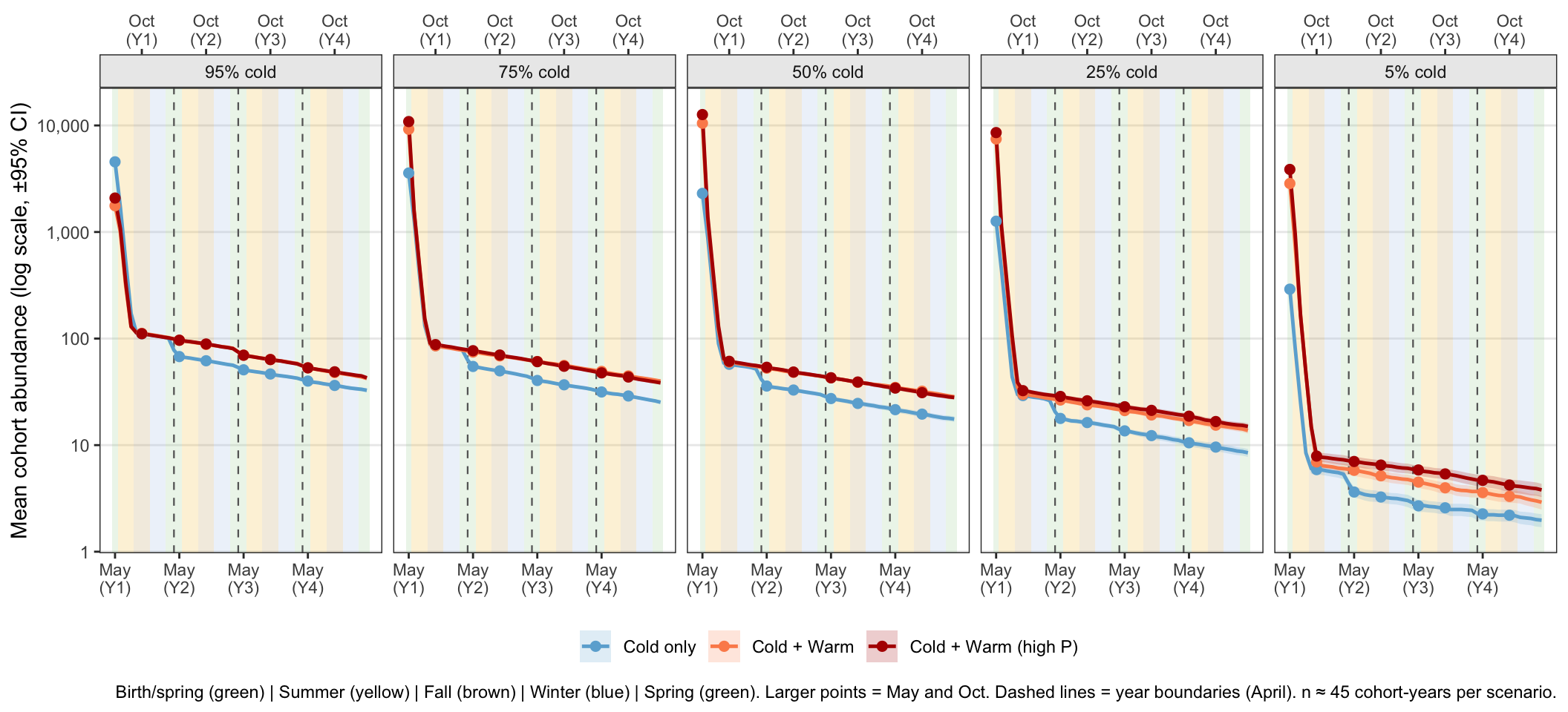
Mean monthly abundance of each birth cohort tracked from hatching through the first four years of life, averaging across all experimental-period cohort-years. The monthly resolution reveals two distinct seasonal survival bottlenecks:
1. a steep summer decline that is common to all simulation runs
2. a winter/spring divergence between scenarios driven declines in abundance for the cold-only scenarios.
```{r cohort-abund-data}
#| cache: true
# ── Helper: monthly cohort abundance from birth through max_months ────────────
f_cohort_ts <- function(df, exp_start, max_months = 48L, birth_mo = 4L) {
  exp_yr  <- year(exp_start)
  max_coh <- exp_yr + 45L
  df |>
    filter(survived == 1L, date >= exp_start, day(date) == 1L) |>
    mutate(
      yr  = year(date),
      mo  = month(date),
      msb = (yr - cohort) * 12L + (mo - birth_mo)  # months since April birth
    ) |>
    filter(msb >= 1L, msb <= max_months,
           cohort >= exp_yr, cohort <= max_coh) |>
    count(cohort, msb, name = "n") |>
    group_by(msb) |>
    summarise(mean_n = mean(n),
              se_n   = sd(n) / sqrt(n()),
              n_coh  = n(),
              .groups = "drop")
}


cohort_ts_df <- bind_rows(lapply(ibm_list_mech, \(s) {
  f_cohort_ts(s$df, exp_start_date) |>
    mutate(prop_cold = s$pc,
           hab_type  = s$ht,
           label     = scen_meta$label[scen_meta$prop_cold == s$pc])
})) |>
  mutate(
    label    = factor(label, levels = scen_meta$label),
    hab_type = factor(hab_type,
                      levels = c("Cold only", "Cold + Warm", "Cold + Warm (high P)"))
  )
```
```{r cohort-abund-plot}
#| fig-width: 11
#| fig-height: 5
# ── Seasonal shading via annotate() — bypasses fill scale entirely ────────────
# Seasons per year: May(1) | Jun-Aug(2-4)=summer | Sep-Nov(5-7)=fall
#                   Dec-Feb(8-10)=winter | Mar-Apr(11-12)=spring
# annotate() draws at fixed coordinates without routing through any fill scale,
# so geom_ribbon can use scale_fill_manual() without conflict.
make_season_layers <- function(n_years = 4L, ymin = 0.1, ymax = 1e7) {
  xmin_tmpl <- c( 0.5,  1.5,  4.5,  7.5, 10.5)
  xmax_tmpl <- c( 1.5,  4.5,  7.5, 10.5, 12.5)
  fill_tmpl <- c("#A8D5A2", "#F5C543", "#C8A96E", "#AEC6E8", "#A8D5A2")
  unlist(lapply(0:(n_years - 1L), \(y)
    lapply(seq_along(fill_tmpl), \(i)
      annotate("rect",
               xmin  = xmin_tmpl[i] + y * 12,
               xmax  = xmax_tmpl[i] + y * 12,
               ymin  = ymin, ymax = ymax,  # finite bounds required (log scale fails with -Inf/Inf)
               fill  = fill_tmpl[i],
               alpha = 0.22)
    )
  ), recursive = FALSE)
}

yr_lines  <- tibble(msb = c(12L, 24L, 36L))
hab_cols  <- c("Cold only"            = "#6BAED6",
               "Cold + Warm"          = "#FC8D59",
               "Cold + Warm (high P)" = "#B30000")


ggplot(cohort_ts_df,
       aes(x = msb, y = mean_n, color = hab_type, group = hab_type)) +
  make_season_layers(4L) +
  geom_vline(data = yr_lines, aes(xintercept = msb),
             inherit.aes = FALSE,
             linetype = "dashed", linewidth = 0.4, color = "grey40") +
  geom_ribbon(aes(ymin = pmax(0.5, mean_n - 1.96 * se_n),
                  ymax = mean_n + 1.96 * se_n,
                  fill = hab_type),
              alpha = 0.20, color = NA) +
  geom_line(linewidth = 0.85) +
  geom_point(data = \(d) filter(d, msb %in% c(1L, 6L, 13L, 18L, 25L, 30L, 37L, 42L)),
             size = 2.0) +
  facet_wrap(~ label, nrow = 1) +
  scale_color_manual(values = hab_cols, name = NULL) +
  scale_fill_manual(values  = hab_cols, name = NULL,
                    breaks  = names(hab_cols)) +
  scale_x_continuous(
    breaks = c(1L, 13L, 25L, 37L),
    labels = c("May\n(Y1)", "May\n(Y2)", "May\n(Y3)", "May\n(Y4)"),
    minor_breaks = NULL,
    sec.axis = sec_axis(~ .,
      breaks = c(6L, 18L, 30L, 42L),
      labels = c("Oct\n(Y1)", "Oct\n(Y2)", "Oct\n(Y3)", "Oct\n(Y4)"))
  ) +
  scale_y_log10(labels = scales::label_comma()) +
  # coord_cartesian clips the view to the data range without affecting the
  # annotate rectangles (which extend to ymax = 1e7 to fill the panel)
  coord_cartesian(ylim = c(
    min(cohort_ts_df$mean_n - 1.96 * cohort_ts_df$se_n, na.rm = TRUE) * 0.9,
    max(cohort_ts_df$mean_n + 1.96 * cohort_ts_df$se_n, na.rm = TRUE) * 1.1
  )) +
  labs(
    x       = NULL,
    y       = "Mean cohort abundance (log scale, \u00b195% CI)",
    caption = paste("Birth/spring (green) | Summer (yellow) | Fall (brown)",
                    "| Winter (blue) | Spring (green).",
                    "Larger points = May and Oct. Dashed lines = year boundaries (April).",
                    "n \u2248 45 cohort-years per scenario.")
  ) +
  theme_bw(base_size = 11) +
  theme(
    panel.grid.minor   = element_blank(),
    panel.grid.major.x = element_blank(),
    strip.background   = element_rect(fill = "grey92"),
    axis.text.x        = element_text(size = 8.5),
    legend.position    = "bottom"
  )
```
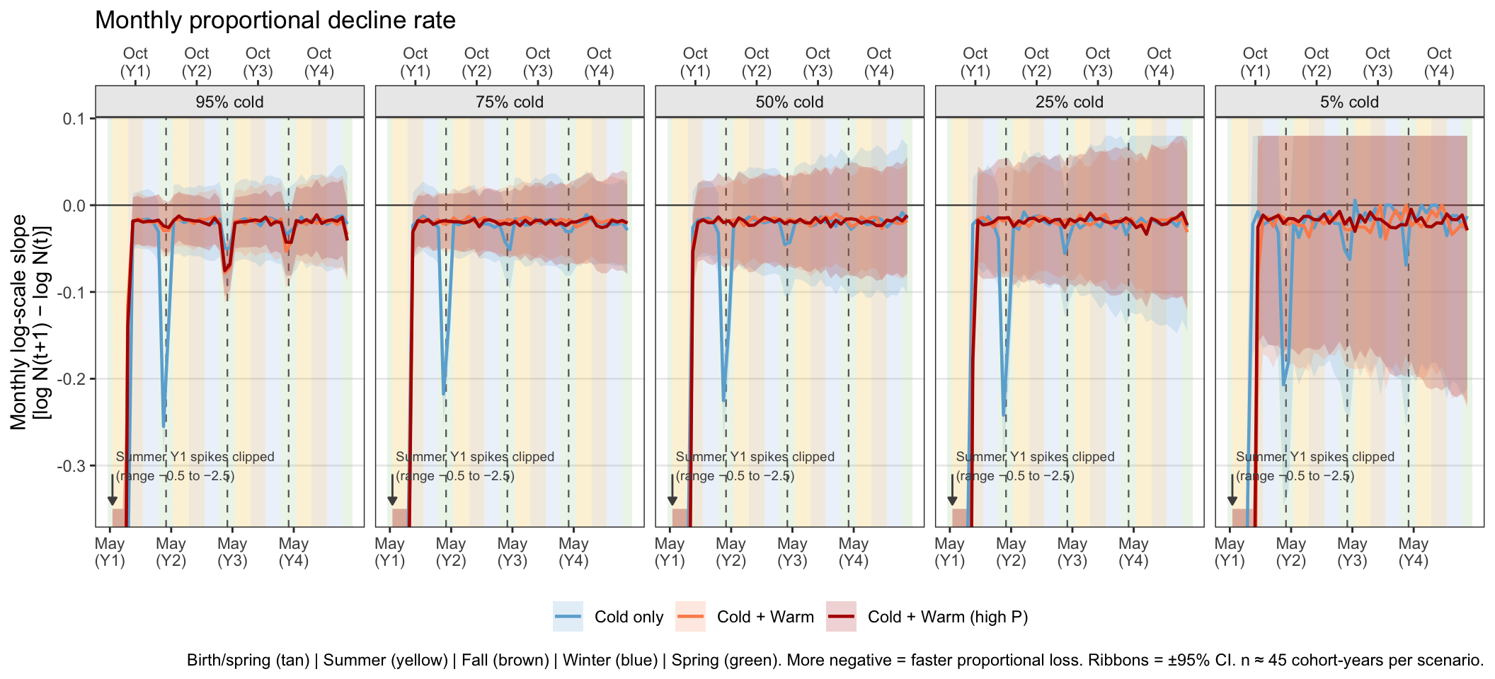
Monthly log-scale slope (the first-difference of log cohort abundance between consecutive monthly snapshots) shows when proportional losses are highest. The y-axis is clipped to reveal post-bottleneck structure; summer Year-1 spikes (birth-pulse to October; range $\approx -0.5$ to $-2.5$) exceed the visible range and are noted with an arrow.
```{r cohort-slope-plot}
#| fig-width: 11
#| fig-height: 5
slope_monthly_df <- cohort_ts_df |>
  arrange(label, hab_type, msb) |>
  group_by(label, hab_type) |>
  mutate(
    msb_mid  = (msb + lead(msb)) / 2,
    slope    = log(lead(mean_n)) - log(mean_n),
    se_slope = sqrt((lead(se_n) / lead(mean_n))^2 + (se_n / mean_n)^2),
    lo95     = slope - 1.96 * se_slope,
    hi95     = slope + 1.96 * se_slope
  ) |>
  filter(!is.na(slope)) |>
  ungroup()

y_clip_lo <- -0.35
y_clip_hi <-  0.08

ggplot(slope_monthly_df,
       aes(x = msb_mid, y = slope, color = hab_type, group = hab_type)) +
  # Seasonal bands: use finite y bounds spanning the clipped axis range
  make_season_layers(4L, ymin = y_clip_lo - 0.05, ymax = y_clip_hi + 0.05) +
  geom_hline(yintercept = 0, linewidth = 0.4, color = "grey30") +
  geom_vline(data = yr_lines, aes(xintercept = msb),
             inherit.aes = FALSE,
             linetype = "dashed", linewidth = 0.4, color = "grey40") +
  geom_ribbon(aes(ymin = pmax(lo95, y_clip_lo),
                  ymax = pmin(hi95, y_clip_hi),
                  fill = hab_type),
              alpha = 0.18, color = NA) +
  geom_line(linewidth = 0.8) +
  # Arrow marking clipped summer spikes
  annotate("segment",
           x = 1.5, xend = 1.5, y = y_clip_lo + 0.04, yend = y_clip_lo + 0.005,
           arrow = arrow(length = unit(0.15, "cm"), type = "closed"),
           color = "grey30") +
  annotate("text", x = 2.2, y = y_clip_lo + 0.05,
           label = "Summer Y1 spikes clipped\n(range \u22120.5 to \u22122.5)",
           size = 2.5, color = "grey30", hjust = 0) +
  facet_wrap(~ label, nrow = 1) +
  scale_color_manual(values = hab_cols, name = NULL) +
  scale_fill_manual(values  = hab_cols, name = NULL,
                    breaks  = names(hab_cols)) +
  scale_x_continuous(
    breaks = c(1L, 13L, 25L, 37L),
    labels = c("May\n(Y1)", "May\n(Y2)", "May\n(Y3)", "May\n(Y4)"),
    minor_breaks = NULL,
    sec.axis = sec_axis(~ .,
      breaks = c(6L, 18L, 30L, 42L),
      labels = c("Oct\n(Y1)", "Oct\n(Y2)", "Oct\n(Y3)", "Oct\n(Y4)"))
  ) +
  scale_y_continuous(labels = scales::label_number(accuracy = 0.1)) +
  coord_cartesian(ylim = c(y_clip_lo, y_clip_hi)) +
  labs(
    x       = NULL,
    y       = "Monthly log-scale slope\n[log N(t+1) \u2212 log N(t)]",
    title   = "Monthly proportional decline rate",
    caption = paste(
      "Birth/spring (tan) | Summer (yellow) | Fall (brown) | Winter (blue) | Spring (green).",
      "More negative = faster proportional loss. Ribbons = \u00b195% CI.",
      "n \u2248 45 cohort-years per scenario."
    )
  ) +
  theme_bw(base_size = 11) +
  theme(
    panel.grid.minor   = element_blank(),
    panel.grid.major.x = element_blank(),
    strip.background   = element_rect(fill = "grey92"),
    axis.text.x        = element_text(size = 8.5),
    legend.position    = "bottom"
  )
```
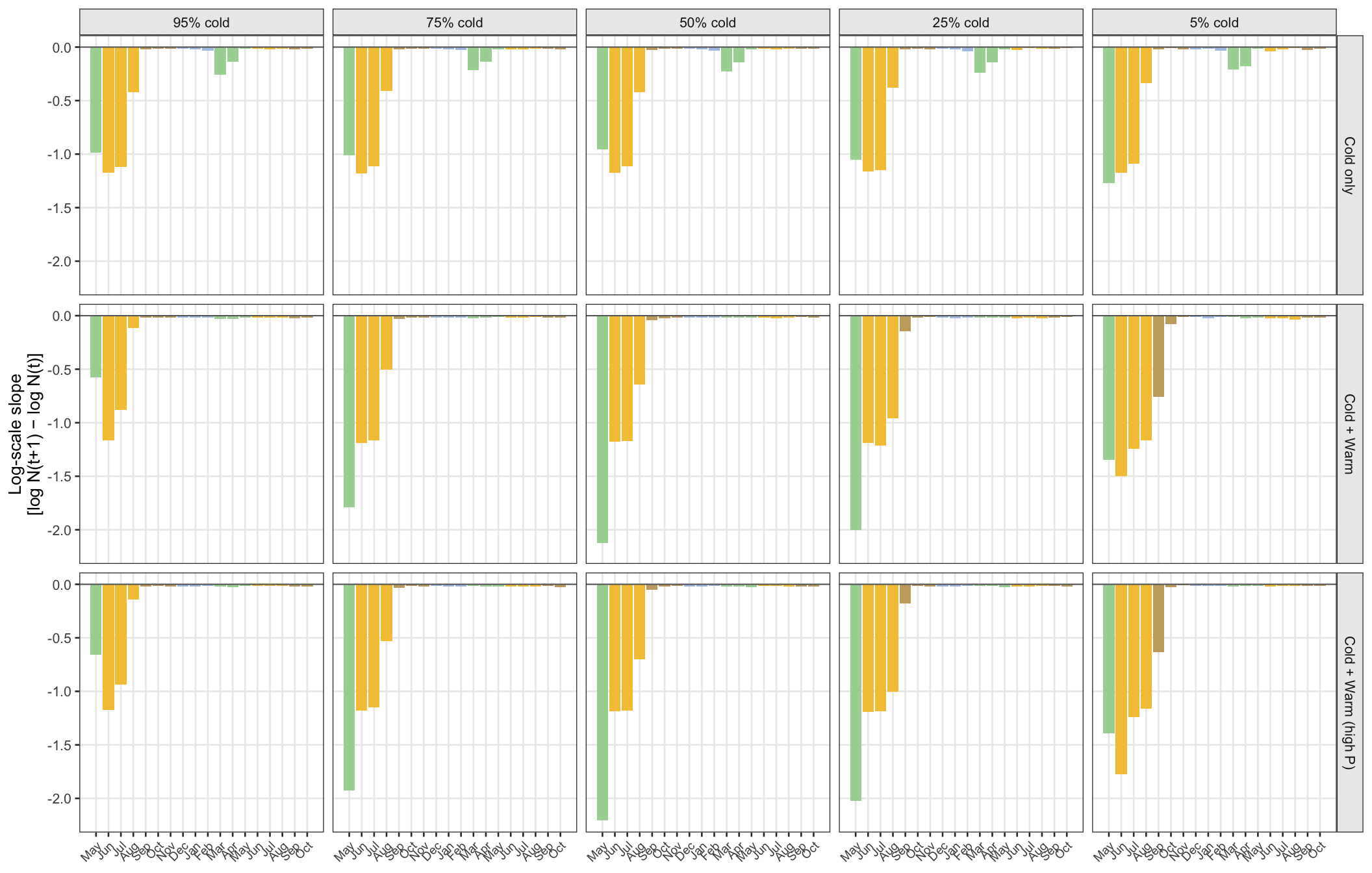
The bar chart below shows raw monthly slopes for the first 18 months of life (birth through October of year 2), preserving the within- and between-year structure to identify which months drive the greatest proportional losses. The plots clearly reveal two demographic bottlenecks: (1) major declines during May-August under all habitat scenarios and cold proportions (this is more severe and extends into September for cold+warm scenarios), and (2) smaller, but significant declines during the following March/April, but only for cold-only scenarios.
```{r slope-month-histogram}
#| fig-width: 11
#| fig-height: 7
# x-axis labels for msb 1–18: Y1 months then Y2 months with suffix
msb_labs_18 <- c(month.abb[c(5:12, 1:4)],
                 month.abb[5:10])

slope_month_hist <- slope_monthly_df |>
  filter(msb <= 18L) |>
  mutate(cal_month = ((msb - 1L + 4L) %% 12L) + 1L,
         mon       = month.abb[cal_month])

# Seasonal fill palette matching make_season_layers shading
mon_fill <- c(
  May = "#A8D5A2",
  Jun = "#F5C543", Jul = "#F5C543", Aug = "#F5C543",
  Sep = "#C8A96E", Oct = "#C8A96E", Nov = "#C8A96E",
  Dec = "#AEC6E8", Jan = "#AEC6E8", Feb = "#AEC6E8",
  Mar = "#A8D5A2", Apr = "#A8D5A2"
)

ggplot(slope_month_hist,
       aes(x = msb, y = slope, fill = mon)) +
  geom_col() +
  geom_hline(yintercept = 0, linewidth = 0.35, color = "grey40") +
  facet_grid(hab_type ~ label) +
  scale_fill_manual(values = mon_fill) +
  scale_x_continuous(breaks = 1:18, labels = msb_labs_18, minor_breaks = NULL) +
  labs(x = NULL,
       y = "Log-scale slope\n[log N(t+1) \u2212 log N(t)]") +
  theme_bw(base_size = 10) +
  theme(panel.grid.minor    = element_blank(),
        # panel.grid.major.x  = element_blank(),
        strip.background    = element_rect(fill = "grey92"),
        axis.text.x         = element_text(size = 7, angle = 45, hjust = 1),
        legend.position     = "none")
```
### Cold habitat availability constrains summer recruitment
#### Fry production
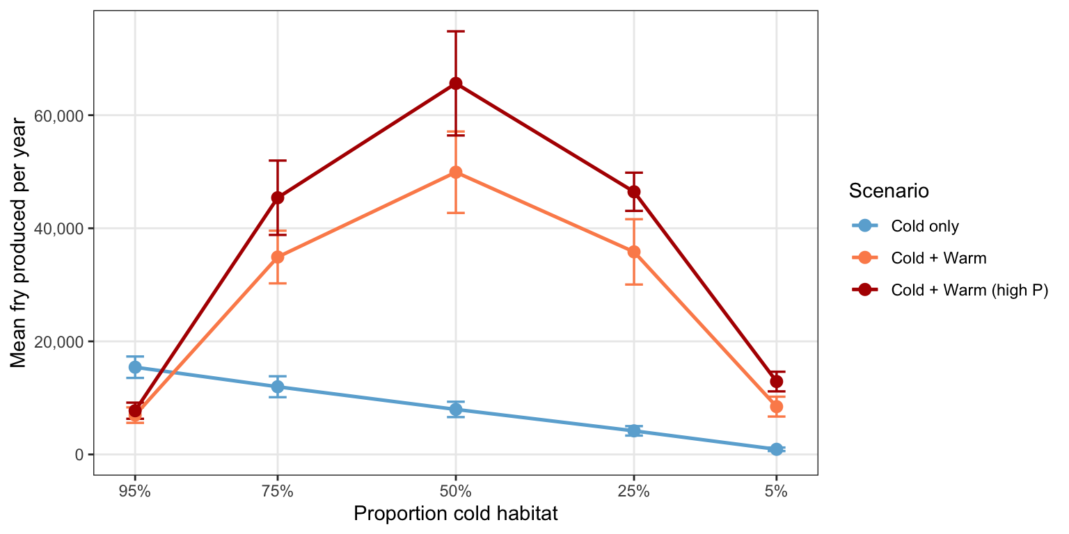
The number of fry produced is a function of adult size and abundance (fecundity), which are driven by warm and cold habitat availability. Importantly, when only cold habitat is available, the number of fry produced declines ~linearly with cold habitat availability. But when warm habitat is also available, considerably more fry are produced at a given proportion cold (except for 95% cold); i.e.,
```{r}
#| cache: false
#| fig-width: 8
#| fig-height: 4
# Single helper computing all reproductive and recruitment metrics in one pass.
# Stored as full_df and reused by both the reproductive output and recruitment
# success figures that follow.
f_repro_recruit <- function(df) {
  exp_df <- df |> filter(date >= exp_start_date)

  fry_birth <- exp_df |>
    filter(!is.na(parent_pid), dayofsim == birth_dayofsim)

  annual <- fry_birth |>
    mutate(yr = year(date)) |>
    group_by(yr) |>
    summarise(n_fry      = n(),
              n_spawners = n_distinct(parent_pid),
              .groups    = "drop") |>
    mutate(fry_per_sp = n_fry / n_spawners)

  nov1_n <- exp_df |>
    filter(month(date) == 11, day(date) == 1, survived == 1) |>
    count(yr = year(date), name = "n_total")

  age0_yr <- exp_df |>
    filter(month(date) == 11, day(date) == 1, survived == 1, floor(age) == 0) |>
    count(yr = year(date), name = "n_age0")

  # Survivors to April 1 of the cohort's first spring. Uses the cohort column
  # to match each fish to their birth year, preventing overlap with the incoming
  # cohort (born Apr–Jun of the new year).
  apr1_age0 <- exp_df |>
    filter(month(date) == 5, day(date) == 1, survived == 1,
           year(date) == cohort + 1L) |>
    count(yr = cohort, name = "n_apr1")

  full <- annual |>
    left_join(nov1_n,   by = "yr") |>
    left_join(age0_yr,  by = "yr") |>
    left_join(apr1_age0, by = "yr") |>
    mutate(
      fry_per_ind    = n_fry      / n_total,
      prop_spawn     = n_spawners / n_total,
      rec_per_sp     = n_age0     / n_spawners,
      rec_per_1k_fry = n_age0     / n_fry * 1000
    )

  tibble(
    mean_n_fry          = mean(full$n_fry,          na.rm = TRUE),
    sd_n_fry            = sd(full$n_fry,            na.rm = TRUE),
    mean_prop_spawn     = mean(full$prop_spawn,     na.rm = TRUE),
    sd_prop_spawn       = sd(full$prop_spawn,       na.rm = TRUE),
    mean_fry_per_sp     = mean(full$fry_per_sp,     na.rm = TRUE),
    sd_fry_per_sp       = sd(full$fry_per_sp,       na.rm = TRUE),
    mean_fry_per_ind    = mean(full$fry_per_ind,    na.rm = TRUE),
    sd_fry_per_ind      = sd(full$fry_per_ind,      na.rm = TRUE),
    mean_birth_wt       = mean(fry_birth$weight,    na.rm = TRUE),
    sd_birth_wt         = sd(fry_birth$weight,      na.rm = TRUE),
    mean_n_age0         = mean(full$n_age0,         na.rm = TRUE),
    sd_n_age0           = sd(full$n_age0,           na.rm = TRUE),
    mean_rec_per_sp     = mean(full$rec_per_sp,     na.rm = TRUE),
    sd_rec_per_sp       = sd(full$rec_per_sp,       na.rm = TRUE),
    mean_rec_per_1k_fry = mean(full$rec_per_1k_fry, na.rm = TRUE),
    sd_rec_per_1k_fry   = sd(full$rec_per_1k_fry,  na.rm = TRUE),
    mean_n_apr1         = mean(full$n_apr1,         na.rm = TRUE),
    sd_n_apr1           = sd(full$n_apr1,           na.rm = TRUE)
  )
}

rows_rr <- vector("list", length(ibm_list_mech))
for (i in seq_along(ibm_list_mech)) {
  s <- ibm_list_mech[[i]]
  rows_rr[[i]] <- f_repro_recruit(s$df) |>
    mutate(prop_cold = s$pc, hab_type = s$ht)
}

full_df <- bind_rows(rows_rr) |>
  mutate(hab_type = factor(hab_type, levels = c("Cold only","Cold + Warm","Cold + Warm (high P)")),
         label    = factor(paste0(prop_cold * 100, "% cold"),
                           levels = pc_labels_mech))

# ── Panel factory ─────────────────────────────────────────────────────────────
mk_panel <- function(df, y, ylo, yhi, ylabel, tag,
                     show_x = FALSE, pct = FALSE) {
  ggplot(df, aes(x = prop_cold, color = hab_type, shape = hab_type)) +
    geom_errorbar(aes(ymin = {{ ylo }}, ymax = {{ yhi }}),
                  width = 0.025, linewidth = 0.6) +
    geom_line(aes(y = {{ y }}), linewidth = 0.9, linetype = "solid") +
    geom_point(aes(y = {{ y }}), size = 3, shape = 16) +
    scale_color_manual(values = hab_cols, name = "Scenario") +
    # scale_shape_manual(values = hab_shp_mech,  name = "Scenario") +
    scale_x_continuous(name   = if (show_x) "Proportion cold habitat" else NULL,
                       breaks = pc_levels_mech,
                       labels = scales::label_percent(accuracy = 1),
                       transform = "reverse") +
    scale_y_continuous(limits = c(0, NA),
                       labels = if (pct) scales::label_percent(accuracy = 1)
                                else     scales::label_number()) +
    labs(y = ylabel, tag = tag) +
    theme_bw() +
    theme(panel.grid.minor = element_blank(),
          legend.position  = "right",
          plot.tag         = element_text(face = "bold"),
          axis.text.x  = if (show_x) element_text() else element_blank(),
          axis.ticks.x = if (show_x) element_line() else element_blank())
}

# ── Reproductive output (5 panels) ───────────────────────────────────────────
mk_panel(full_df,
  mean_n_fry, pmax(mean_n_fry - sd_n_fry, 0), mean_n_fry + sd_n_fry,
  "Mean fry produced per year", NULL, show_x = TRUE) +
  scale_y_continuous(limits = c(0, NA), labels = scales::label_comma())
# rB <- mk_panel(full_df,
#   mean_prop_spawn, pmax(mean_prop_spawn - sd_prop_spawn, 0),
#   mean_prop_spawn + sd_prop_spawn,
#   "Spawning participation\n(spawners / Oct 1 N)", "B", pct = TRUE)
#
# rC <- mk_panel(full_df,
#   mean_fry_per_sp, pmax(mean_fry_per_sp - sd_fry_per_sp, 0),
#   mean_fry_per_sp + sd_fry_per_sp,
#   "Mean fry per spawner", "C")
#
# rD <- mk_panel(full_df,
#   mean_fry_per_ind, pmax(mean_fry_per_ind - sd_fry_per_ind, 0),
#   mean_fry_per_ind + sd_fry_per_ind,
#   "Mean fry per individual\n(Oct 1 census)", "D")
#
# rE <- mk_panel(full_df,
#   mean_birth_wt, pmax(mean_birth_wt - sd_birth_wt, 0),
#   mean_birth_wt + sd_birth_wt,
#   "Mean offspring\nbirth weight (g)", "E", show_x = TRUE)
#
# (rA / rB / rC / rD / rE) +
#   plot_layout(guides = "collect") &
#   theme(legend.position  = "top",
#         legend.key.width = unit(1.2, "cm"))
```
#### Habitat use
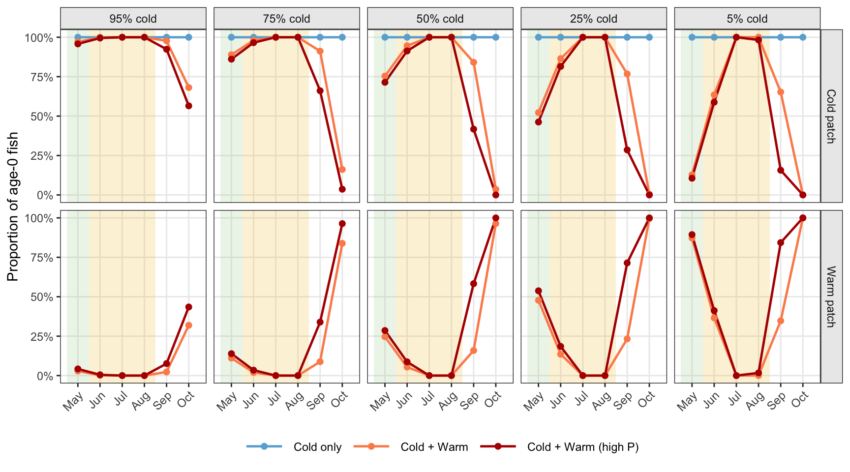
Fish preferentially occupy the cold patch during summer (particularly July and August) to avoid sub-optimally warm temperatures and asssociated metabolic and survival costs in the warm patch.
```{r hab-use-age0-data}
#| cache: true
# Monthly mean age-0 density and patch-use proportion across the full first year
# of life (May–Apr) for each scenario, using cohort year to avoid overlap between
# new cohort fish (born Apr–Jun) and the prior cohort's winter fish.
# msb = months since April birth: May = 1, Jun = 2, ..., Apr = 12.
hab_use_age0 <- bind_rows(lapply(ibm_list_mech, \(s) {
  a_cold  <- s$pc * 2.0
  a_warm  <- (1 - s$pc) * 2.0
  patches <- if (s$ht == "Cold only") "cold" else c("cold", "warm")

  counts <- s$df |>
    filter(date >= exp_start_date) |>
    mutate(
      yr  = year(date),
      mo  = month(date),
      msb = (yr - cohort) * 12L + (mo - 4L)  # months since April birth; May = 1
    ) |>
    filter(msb >= 1L, msb <= 12L) |>           # full first year, no cohort overlap
    count(cohort, msb, patch, name = "n") |>
    complete(nesting(cohort, msb), patch = patches, fill = list(n = 0L))

  tot <- counts |>
    group_by(cohort, msb) |>
    summarise(n_total = sum(n), .groups = "drop")

  counts |>
    left_join(tot, by = c("cohort", "msb")) |>
    mutate(
      area      = if_else(patch == "cold", a_cold, a_warm),
      density   = n / area,
      prop      = if_else(n_total > 0L, n / n_total, NA_real_),
      patch_lab = if_else(patch == "cold", "Cold patch", "Warm patch")
    ) |>
    group_by(msb, patch_lab) |>
    summarise(
      mean_density = mean(density, na.rm = TRUE),
      mean_prop    = mean(prop, na.rm = TRUE),
      .groups      = "drop"
    ) |>
    mutate(
      prop_cold = s$pc,
      hab_type  = s$ht,
      label     = scen_meta$label[scen_meta$prop_cold == s$pc]
    )
})) |>
  mutate(
    patch_lab = factor(patch_lab, levels = c("Cold patch", "Warm patch")),
    label     = factor(label, levels = scen_meta$label),
    hab_type  = factor(hab_type,
                       levels = c("Cold only", "Cold + Warm", "Cold + Warm (high P)"))
  )

# Convenience label vector: May through April
age0_msb_labs <- c(month.abb[5:12], month.abb[1:4])
```
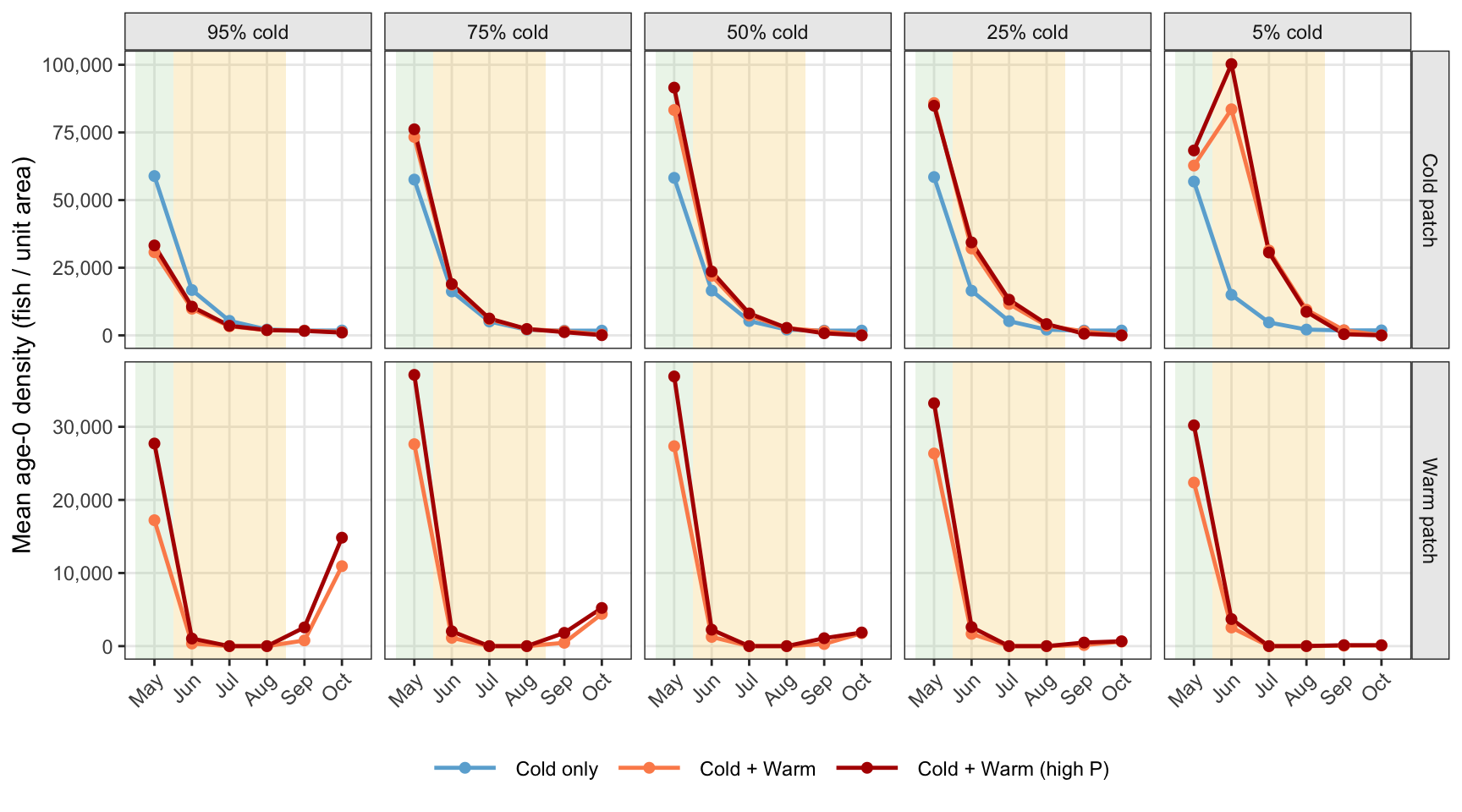
Looking at raw age-0 densities doesn't give us much information, as temporal declines in density are largely driven by declines in total age-0 abundance due to low daily survival probability.
```{r hab-use-summer-density}
#| fig-width: 9
#| fig-height: 5
ggplot(hab_use_age0 |> filter(msb <= 6L),
       aes(x = msb, y = mean_density, color = hab_type, group = hab_type)) +
  make_season_layers(4L, ymin = -Inf, ymax = Inf) +
  geom_line(linewidth = 0.85) +
  geom_point(size = 1.8) +
  facet_grid(patch_lab ~ label, scales = "free_y") +
  scale_color_manual(values = hab_cols, name = NULL) +
  scale_x_continuous(breaks = 1:6, labels = month.abb[c(5:10)],
                     minor_breaks = NULL, limits = c(0.5, 6.5)) +
  scale_y_continuous(limits = c(0, NA), labels = scales::label_comma()) +
  labs(x = NULL, y = "Mean age-0 density (fish / unit area)") +
  theme_bw(base_size = 11) +
  theme(panel.grid.minor   = element_blank(),
        strip.background   = element_rect(fill = "grey92"),
        axis.text.x        = element_text(size = 9, angle = 45, hjust = 1),
        legend.position    = "bottom",
        legend.key.width   = unit(1.2, "cm"))
```
But if we look at the proportion of the age-0 population using either cold or warm patches, we can see that fish flood into the cold patch during summer (particularly July and August), avoiding the warm patch even when warm patch area is relatively high. As the proportion of habitat that is cold declines, greater proportions of fish use the warm habitat during the shoulder seasons (May-June and Sept-Oct) as density dependent constraints on growth are relieved and the scope for growth increases. This pattern is magnified when higher consumption is allowed in the warm habitat.
```{r hab-use-summer-prop}
#| fig-width: 9
#| fig-height: 5
ggplot(hab_use_age0 |> filter(msb <= 6L),
       aes(x = msb, y = mean_prop, color = hab_type, group = hab_type)) +
  make_season_layers(4L, ymin = -Inf, ymax = Inf) +
  geom_line(linewidth = 0.85) +
  geom_point(size = 1.8) +
  facet_grid(patch_lab ~ label) +
  scale_color_manual(values = hab_cols, name = NULL) +
  scale_x_continuous(breaks = 1:6, labels = month.abb[c(5:10)],
                     minor_breaks = NULL, limits = c(0.5, 6.5)) +
  scale_y_continuous(limits = c(0, 1),
                     labels = scales::label_percent(accuracy = 1)) +
  labs(x = NULL, y = "Proportion of age-0 fish") +
  theme_bw(base_size = 11) +
  theme(panel.grid.minor   = element_blank(),
        strip.background   = element_rect(fill = "grey92"),
        axis.text.x        = element_text(size = 9, angle = 45, hjust = 1),
        legend.position    = "bottom",
        legend.key.width   = unit(1.2, "cm"))
```
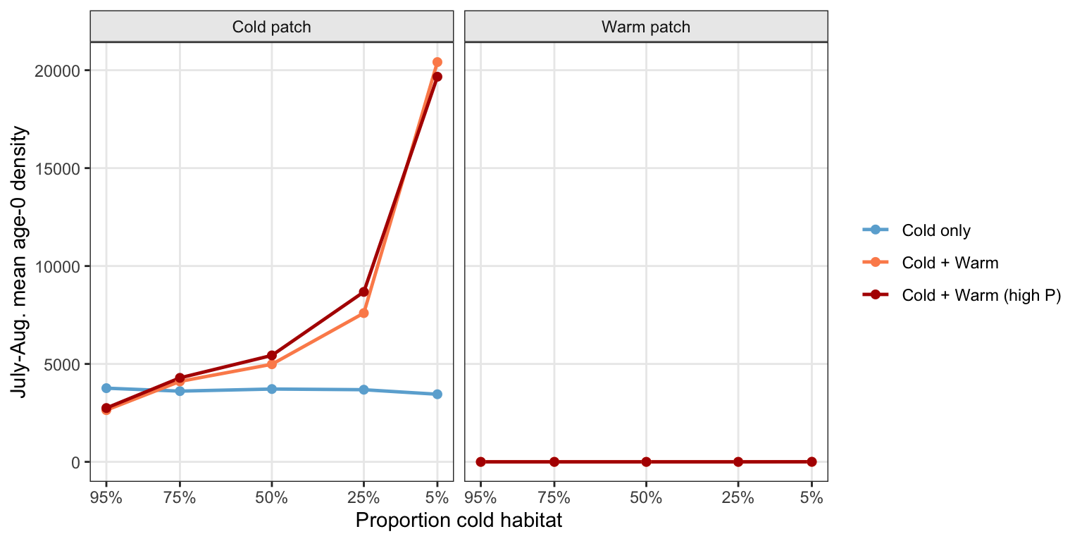
In summary, fish are preferrentially using the cold patch during summer, regardless of cold proportion. Summer densities are greater in the cold patch than in the warm patch, and this difference is magnified as the proportion of cold habitat declines. Furthermore, cold patch summer densities are *almost* always greater in cold+warm relative to cold-only scenarios.
```{r}
#| fig-width: 8
#| fig-height: 4
hab_use_age0 |> filter(msb %in% c(3:4)) |> group_by(prop_cold, hab_type, label, patch_lab) |> summarise(mean_density = mean(mean_density)) |> ungroup() |>
  ggplot(aes(x = prop_cold, y = mean_density, color = hab_type, group = hab_type)) +
  geom_line(linewidth = 0.85) +
  geom_point(size = 1.8) +
  facet_wrap(~patch_lab, nrow = 1) +
  scale_color_manual(values = hab_cols, name = NULL) +
  scale_x_reverse(breaks = pc_levels,
                  labels = scales::percent_format(accuracy = 1)) +
  # scale_y_continuous(limits = c(0, 1),
  #                    labels = scales::label_number(accuracy = 0.1)) +
  labs(x = "Proportion cold habitat", y = "July-Aug. mean age-0 density") +
  theme_bw(base_size = 11) +
  theme(panel.grid.minor   = element_blank(),
        strip.background   = element_rect(fill = "grey92"),
        # axis.text.x        = element_text(size = 9, angle = 45, hjust = 1),
        legend.position    = "right")
```
#### Density dependence
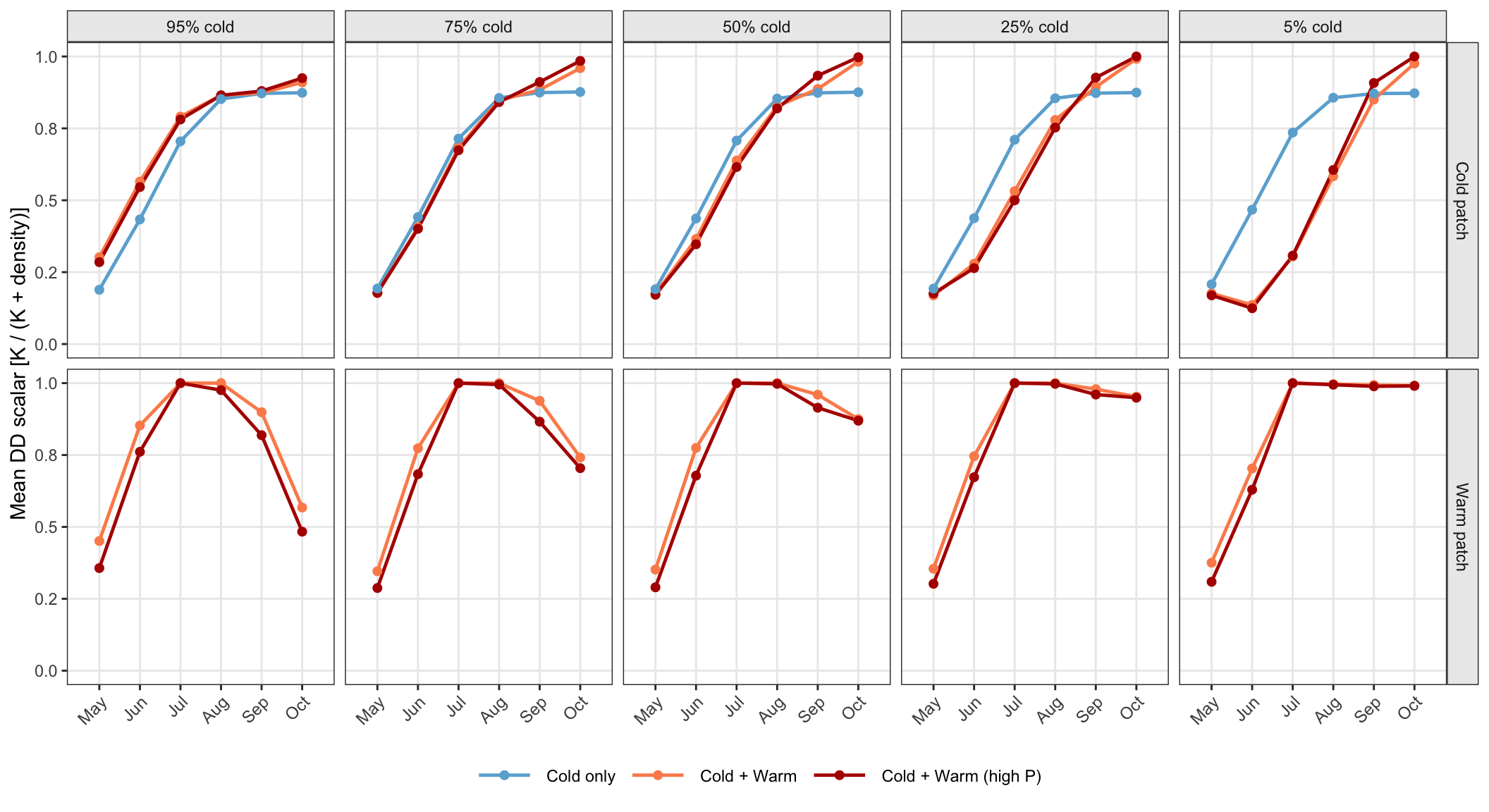
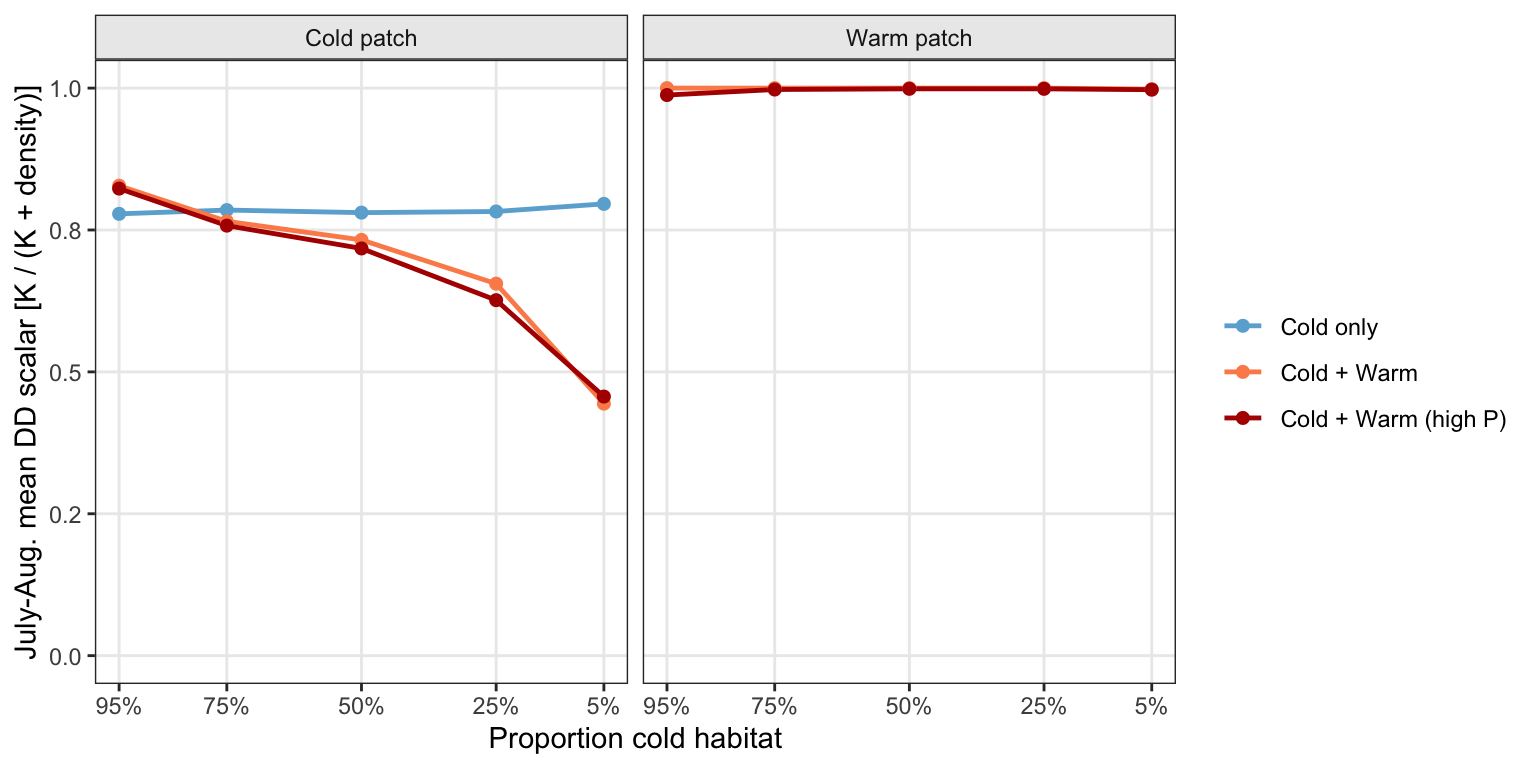
As a result of a larger number of fish using a fixed amount of (cold) habitat, the strength of density dependence during the first summer (particularly July-August) is much stronger (lower DD scalar) for the cold+warm scenarios relative to the cold-only scenarios, and this effect is more pronounced as the cold patch shrinks. The strength of density dependence in the warm patch (for the cold-warm scenarios) is low (high DD scalar) and does not vary with cold/warm patch proportion, as very few/no fish are using the warm patch at this time.
```{r dd-age0-data}
#| cache: true
# Monthly mean DD scalar experienced by age-0 fish, by patch, full first year
# (May–Apr, msb 1–12). Cohort-aware msb prevents mixing new-cohort fry (born
# Apr–Jun) into the prior cohort's late-winter months.
# K = 400 per unit area; a_cold = pc * 2, a_warm = (1 - pc) * 2.
dd_age0_df <- bind_rows(lapply(ibm_list_mech, \(s) {
  a_cold <- s$pc * 2.0
  a_warm <- (1 - s$pc) * 2.0

  cold_dd <- s$df |>
    filter(date >= exp_start_date, patch == "cold") |>
    mutate(
      yr  = year(date),
      mo  = month(date),
      msb = (yr - cohort) * 12L + (mo - 4L)
    ) |>
    filter(msb >= 1L, msb <= 12L) |>
    count(date, msb, name = "n") |>
    mutate(dd = 400 / (400 + n / a_cold)) |>
    group_by(msb) |>
    summarise(mean_dd = mean(dd), .groups = "drop") |>
    mutate(patch_lab = "Cold patch")

  out <- cold_dd

  if (a_warm > 0) {
    warm_dd <- s$df |>
      filter(date >= exp_start_date, patch == "warm") |>
      mutate(
        yr  = year(date),
        mo  = month(date),
        msb = (yr - cohort) * 12L + (mo - 4L)
      ) |>
      filter(msb >= 1L, msb <= 12L) |>
      count(date, msb, name = "n") |>
      mutate(dd = 400 / (400 + n / a_warm)) |>
      group_by(msb) |>
      summarise(mean_dd = mean(dd), .groups = "drop") |>
      mutate(patch_lab = "Warm patch")
    out <- bind_rows(cold_dd, warm_dd)
  }

  out |>
    mutate(
      prop_cold = s$pc,
      hab_type  = s$ht,
      label     = scen_meta$label[scen_meta$prop_cold == s$pc]
    )
})) |>
  # Fill months with no age-0 fish in a patch with DD = 1 (no density dependence).
  complete(nesting(prop_cold, hab_type, label, patch_lab), msb = 1:12,
           fill = list(mean_dd = 1)) |>
  mutate(
    patch_lab = factor(patch_lab, levels = c("Cold patch", "Warm patch")),
    label     = factor(label, levels = scen_meta$label),
    hab_type  = factor(hab_type,
                       levels = c("Cold only", "Cold + Warm", "Cold + Warm (high P)"))
  )
```
```{r dd-summer-plot}
#| fig-width: 11
#| fig-height: 6
ggplot(dd_age0_df |> filter(msb <= 6L),
       aes(x = msb, y = mean_dd, color = hab_type, group = hab_type)) +
  # make_season_layers(1L, ymin = 0, ymax = 1) +
  geom_line(linewidth = 0.85) +
  geom_point(size = 1.8) +
  facet_grid(patch_lab ~ label) +
  scale_color_manual(values = hab_cols, name = NULL) +
  scale_x_continuous(breaks = 1:6, labels = month.abb[5:10],
                     minor_breaks = NULL, limits = c(0.5, 6.5)) +
  scale_y_continuous(limits = c(0, 1),
                     labels = scales::label_number(accuracy = 0.1)) +
  labs(x = NULL, y = "Mean DD scalar [K / (K + density)]") +
  theme_bw(base_size = 11) +
  theme(panel.grid.minor   = element_blank(),
        strip.background   = element_rect(fill = "grey92"),
        axis.text.x        = element_text(size = 9, angle = 45, hjust = 1),
        legend.position    = "bottom",
        legend.key.width   = unit(1.2, "cm"))
```
```{r}
#| fig-width: 8
#| fig-height: 4
#|
dd_age0_df |> filter(msb %in% c(3:4)) |> group_by(prop_cold, hab_type, label, patch_lab) |> summarise(mean_dd = mean(mean_dd)) |> ungroup() |>
  ggplot(aes(x = prop_cold, y = mean_dd, color = hab_type, group = hab_type)) +
  geom_line(linewidth = 0.85) +
  geom_point(size = 1.8) +
  facet_wrap(~patch_lab, nrow = 1) +
  scale_color_manual(values = hab_cols, name = NULL) +
  scale_x_reverse(breaks = pc_levels,
                  labels = scales::percent_format(accuracy = 1)) +
  scale_y_continuous(limits = c(0, 1),
                     labels = scales::label_number(accuracy = 0.1)) +
  labs(x = "Proportion cold habitat", y = "July-Aug. mean DD scalar [K / (K + density)]") +
  theme_bw(base_size = 11) +
  theme(panel.grid.minor   = element_blank(),
        strip.background   = element_rect(fill = "grey92"),
        # axis.text.x        = element_text(size = 9, angle = 45, hjust = 1),
        legend.position    = "right")
```
#### Consumption
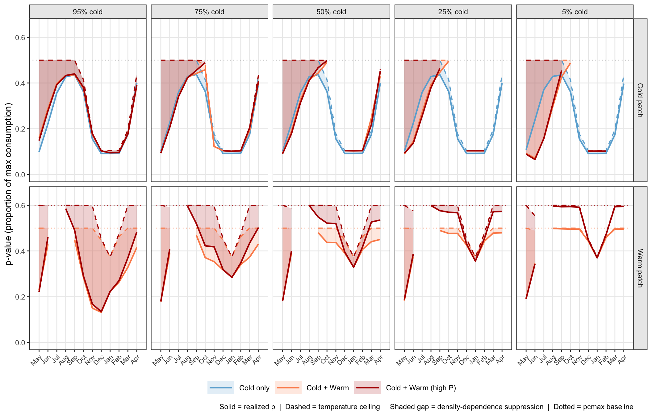
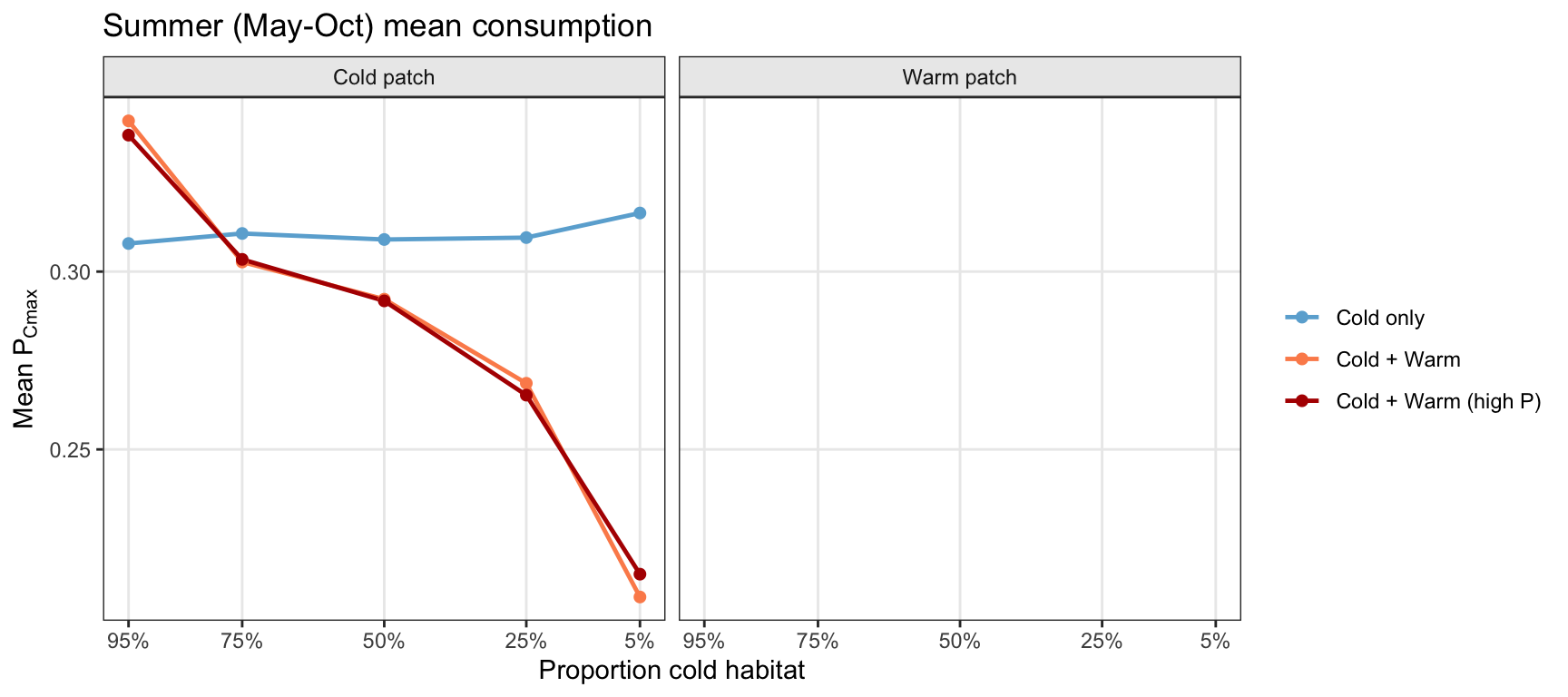
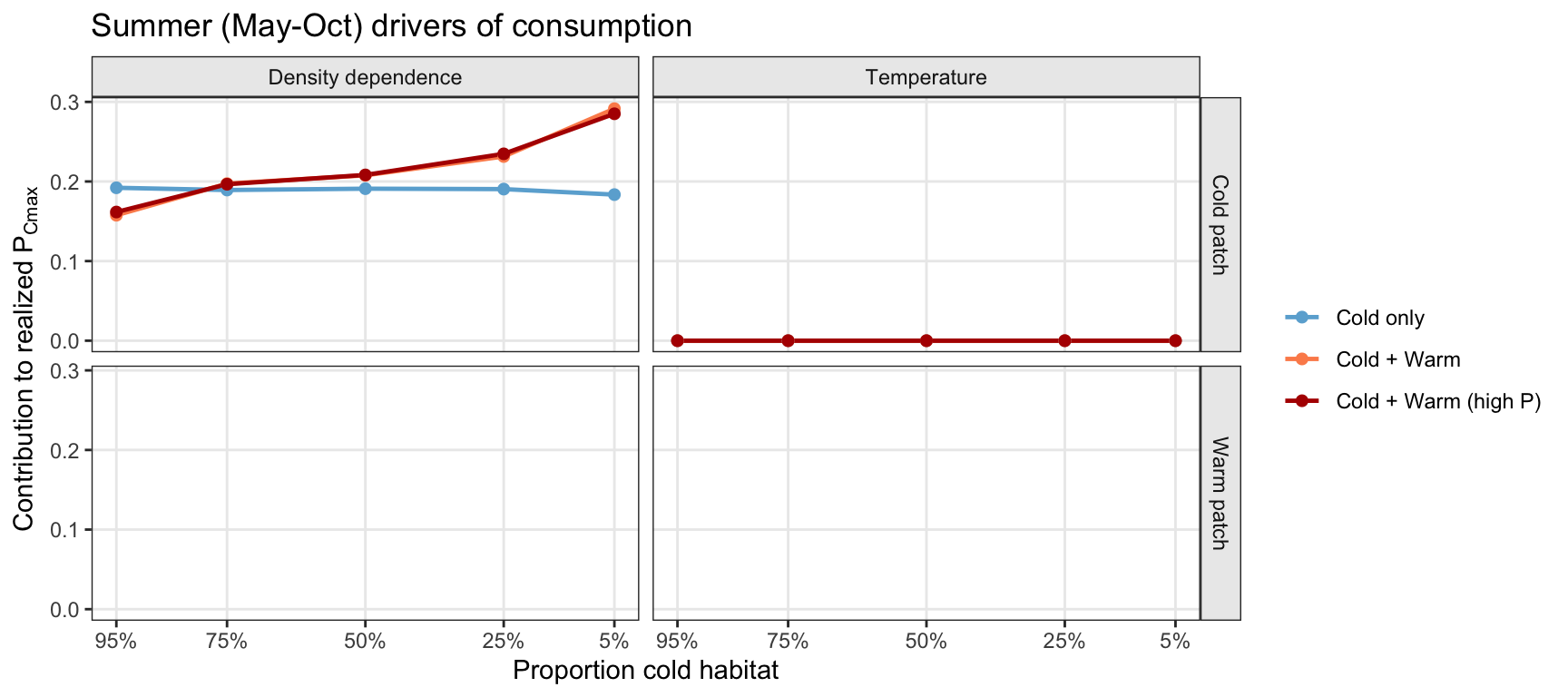
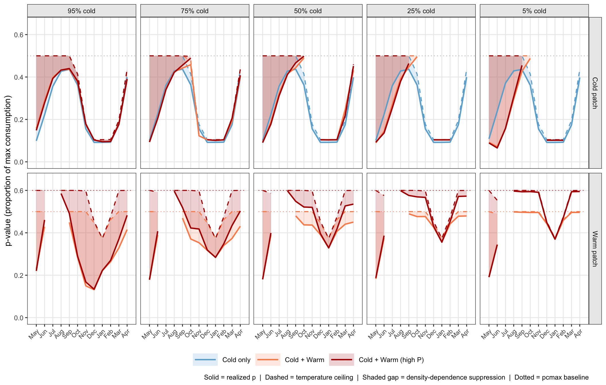
During summer, strong density dependence constrains consumption in the cold patch, whereas temperature plays a comparatively minor role. Density-dependent constraints on consumption in the cold-patch become more severe as cold habitat is increasingly replaced by warm habitat (for cold+warm scenarios...increasing fry production per unit area of cold).
```{r pcmax-age0-data}
#| cache: true
# Monthly mean realized p-value (proportion of maximum consumption) for age-0
# fish, full first year (May–Apr, msb 1–12). Realized p-value combines two
# sequential constraints applied in the simulation:
#   (1) Temperature limitation: pcmax_adj = min(fncTempDepend(temp), pcmax_baseline)
#       Temperature becomes binding below ~7°C, suppressing winter cold-patch
#       consumption independently of density.
#   (2) Density dependence: dd_scalar = K / (K + n / area)
#       Using the same population-level count as dd_age0_df; note the simulation
#       uses per-fish effective density (dominance-adjusted) but the patch-average
#       is appropriate for scenario comparisons.
#   realized_p = pcmax_adj * dd_scalar
#
# fncTempDepend() and base_params are sourced from Functions.qmd / SimulationLoop.qmd.
pcmax_age0_df <- bind_rows(lapply(ibm_list_mech, \(s) {
  a_cold <- s$pc * 2.0
  a_warm <- (1 - s$pc) * 2.0
  K      <- base_params$K_cold  # K_cold == K_warm == 400

  make_pcmax <- function(patch_df, pcmax_b, area, lab) {
    patch_df |>
      filter(date >= exp_start_date, survived == 1L) |>
      mutate(
        yr  = year(date),
        mo  = month(date),
        msb = (yr - cohort) * 12L + (mo - 4L)
      ) |>
      filter(msb >= 1L, msb <= 12L) |>
      group_by(date, msb) |>
      summarise(
        n        = n(),
        temp_day = first(temp),   # patch temperature is shared by all fish
        .groups  = "drop"
      ) |>
      mutate(
        pcmax_adj  = pmin(fncTempDepend(temp_day), pcmax_b),
        dd_scalar  = K / (K + n / area),
        realized_p = pcmax_adj * dd_scalar
      ) |>
      group_by(msb) |>
      summarise(
        mean_realized_p = mean(realized_p),
        mean_pcmax_adj  = mean(pcmax_adj),   # temperature-only constraint
        mean_dd         = mean(dd_scalar),   # density-only constraint
        .groups = "drop"
      ) |>
      mutate(patch_lab = lab)
  }

  out <- make_pcmax(
    s$df |> filter(patch == "cold"),
    s$pcmax_cold, a_cold, "Cold patch"
  )

  if (a_warm > 0) {
    out <- bind_rows(out,
      make_pcmax(
        s$df |> filter(patch == "warm"),
        s$pcmax_warm, a_warm, "Warm patch"
      )
    )
  }

  out |>
    mutate(
      prop_cold = s$pc,
      hab_type  = s$ht,
      label     = scen_meta$label[scen_meta$prop_cold == s$pc]
    )
})) |>
  complete(nesting(prop_cold, hab_type, label, patch_lab), msb = 1:12,
           fill = list(mean_realized_p = NA_real_,
                       mean_pcmax_adj  = NA_real_,
                       mean_dd         = NA_real_)) |>
  mutate(
    patch_lab = factor(patch_lab, levels = c("Cold patch", "Warm patch")),
    label     = factor(label, levels = scen_meta$label),
    hab_type  = factor(hab_type,
                       levels = c("Cold only", "Cold + Warm", "Cold + Warm (high P)"))
  ) |>
  mutate(dd_gap   = mean_pcmax_adj - mean_realized_p,
         temp_gap = ifelse(hab_type == "Cold + Warm (high P)" & patch_lab == "Warm patch", 0.6, 0.5) - mean_pcmax_adj)
```
```{r pcmax-decomp}
#| fig-width: 11
#| fig-height: 7
# Decomposition of realized p-value into temperature and density-dependence
# components across the full age-0 year, for both cold and warm patches.
#   Dashed line  = mean_pcmax_adj  (temperature ceiling; DD removed)
#   Solid line   = mean_realized_p (after DD suppression)
#   Shaded gap   = density-dependence suppression alone
# Cold patch: DD gap widens in early summer for cold+warm scenarios (more fish
#   from warm-enabled reproduction flooding into cold habitat).
# Warm patch: temperature ceiling collapses near peak summer (~Jul–Aug) as
#   fncTempDepend approaches 0 near 24°C, independently of density. Cold-only
#   scenarios have no warm patch and are absent from the bottom row.
# Per-patch, per-hab_type pcmax baseline reference lines.
# Cold patch: single dotted line at 0.5 (same for all scenarios).
# Warm patch: color-coded dotted lines at 0.5 (Cold + Warm) and 0.6 (high P).
pcmax_refs <- data.frame(
  patch_lab  = c("Cold patch", "Warm patch",   "Warm patch"),
  hab_type   = c(NA_character_, "Cold + Warm", "Cold + Warm (high P)"),
  pcmax_base = c(0.5,           0.5,            0.6)
)

pcmax_age0_df |>
  ggplot(aes(x = msb, color = hab_type, fill = hab_type, group = hab_type)) +
  geom_hline(data = pcmax_refs |> filter(is.na(hab_type)),
             aes(yintercept = pcmax_base), inherit.aes = FALSE,
             color = "grey70", linetype = "dotted", linewidth = 0.4) +
  geom_segment(data = pcmax_refs |> filter(!is.na(hab_type)),
               aes(x = 0.5, xend = 12.5,
                   y = pcmax_base, yend = pcmax_base, color = hab_type),
               inherit.aes = FALSE,
               linetype = "dotted", linewidth = 0.4) +
  geom_ribbon(aes(ymin = mean_realized_p, ymax = mean_pcmax_adj),
              alpha = 0.18, color = NA) +
  geom_line(aes(y = mean_pcmax_adj), linetype = "dashed", linewidth = 0.65) +
  geom_line(aes(y = mean_realized_p), linewidth = 0.85) +
  facet_grid(patch_lab ~ label) +
  scale_color_manual(values = hab_cols, name = NULL) +
  scale_fill_manual(values  = hab_cols, name = NULL, breaks = names(hab_cols)) +
  scale_x_continuous(breaks = 1:12, labels = age0_msb_labs, minor_breaks = NULL) +
  scale_y_continuous(limits = c(0, 0.65),
                     labels = scales::label_number(accuracy = 0.1)) +
  labs(x = NULL,
       y = "p-value (proportion of max consumption)",
       caption = "Solid = realized p  |  Dashed = temperature ceiling  |  Shaded gap = density-dependence suppression  |  Dotted = pcmax baseline") +
  theme_bw(base_size = 11) +
  theme(panel.grid.minor   = element_blank(),
        strip.background   = element_rect(fill = "grey92"),
        axis.text.x        = element_text(size = 8, angle = 45, hjust = 1),
        legend.position    = "bottom",
        legend.key.width   = unit(1.2, "cm"))
```
```{r}
#| fig-width: 9
#| fig-height: 4
#|
pcmax_age0_df %>%
  filter(msb %in% c(1:5)) %>%
  mutate(season = ifelse(msb %in% c(1:6), "summer", "winter")#,
         # dd_gap = replace_na(dd_gap, 0),
         # temp_gap = replace_na(temp_gap, 0)
         ) %>%
  filter(season == "summer") %>%
  group_by(prop_cold, hab_type, patch_lab, season) %>%
  summarize(mean_realized_p = mean(mean_realized_p)) %>%
  ungroup() %>%
  ggplot(aes(x = prop_cold, y = mean_realized_p, group = hab_type, color = hab_type)) +
  geom_line(linewidth = 0.85) +
  geom_point(size = 1.8) +
  facet_wrap(~patch_lab) +
  scale_color_manual(values = hab_cols, name = NULL) +
  scale_x_reverse(breaks = pc_levels,
                  labels = scales::percent_format(accuracy = 1)) +
  # scale_y_continuous(limits = c(0, 0.6)) +
  labs(x = "Proportion cold habitat", y = expression(Mean~P[Cmax]),
       title = "Summer (May-Oct) mean consumption") +
  theme_bw(base_size = 11) +
  theme(panel.grid.minor   = element_blank(),
        strip.background   = element_rect(fill = "grey92"),
        # axis.text.x        = element_text(size = 9, angle = 45, hjust = 1),
        legend.position    = "right")
pcmax_age0_df %>%
  filter(msb %in% c(1:5)) %>%
  mutate(season = ifelse(msb %in% c(1:6), "summer", "winter")#,
         # dd_gap = replace_na(dd_gap, 0),
         # temp_gap = replace_na(temp_gap, 0)
         ) %>%
  group_by(prop_cold, hab_type, patch_lab, season) %>%
  summarize(mean_dd_gap = mean(dd_gap),
            mean_temp_gap = mean(temp_gap)) %>%
  ungroup() %>%
  filter(season == "summer") %>%
  gather(mean_dd_gap:mean_temp_gap, key = "driver", value = "mean_gap") %>%
  mutate(driver = recode(driver, "mean_dd_gap" = "Density dependence", "mean_temp_gap" = "Temperature")) %>%
  ggplot(aes(x = prop_cold, y = mean_gap, group = hab_type, color = hab_type)) +
  geom_line(linewidth = 0.85) +
  geom_point(size = 1.8) +
  facet_grid(patch_lab~driver) +
  scale_color_manual(values = hab_cols, name = NULL) +
  scale_x_reverse(breaks = pc_levels,
                  labels = scales::percent_format(accuracy = 1)) +
    # scale_y_continuous(limits = c(0, 0.25)) +
  labs(x = "Proportion cold habitat", y = expression(Contribution~to~realized~P[Cmax]),
       title = "Summer (May-Oct) drivers of consumption") +
  theme_bw(base_size = 11) +
  theme(panel.grid.minor   = element_blank(),
        strip.background   = element_rect(fill = "grey92"),
        # axis.text.x        = element_text(size = 9, angle = 45, hjust = 1),
        legend.position    = "right")
```
#### Growth
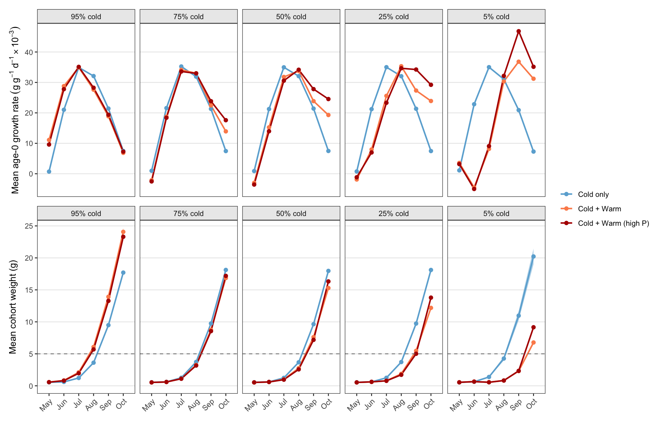
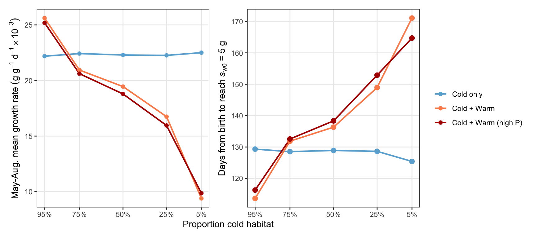
Mean summer age-0 growth rates thus decline as the cold patch shrinks (for the cold+warm scenarios), but are unaffected by cold patch availability when only cold habitat is available. Similarly, the time it takes age-0 fish to clear the size-based survival threshold (5 g) increases as the cold patch shrinks (for cold-warm scenarios), owing to slower overall growth during summer.
```{r gr-size-age0-data}
#| cache: true
# ── Plot A: monthly mean ggd for living age-0 fish, full first year (May–Apr) ─
# Cohort-aware msb prevents mixing new-cohort fry into the prior cohort's
# late-winter months. survived == 1L: fish alive on each day.
gr_age0_df <- bind_rows(lapply(ibm_list_mech, \(s) {
  s$df |>
    filter(date >= exp_start_date, survived == 1L, !is.na(ggd)) |>
    mutate(
      yr  = year(date),
      mo  = month(date),
      msb = (yr - cohort) * 12L + (mo - 4L)
    ) |>
    filter(msb >= 1L, msb <= 12L) |>
    group_by(msb) |>
    summarise(mean_ggd = mean(ggd) * 1000, .groups = "drop") |>
    mutate(prop_cold = s$pc,
           hab_type  = s$ht,
           label     = scen_meta$label[scen_meta$prop_cold == s$pc])
})) |>
  mutate(
    label    = factor(label, levels = scen_meta$label),
    hab_type = factor(hab_type,
                      levels = c("Cold only", "Cold + Warm", "Cold + Warm (high P)"))
  )

# ── Plot B: mean cohort weight trajectories, full first year (msb 1–12) ───────
wt_age0_df <- bind_rows(lapply(ibm_list_mech, \(s) {
  exp_yr  <- year(exp_start_date)
  max_coh <- exp_yr + 45L
  s$df |>
    filter(survived == 1L, date >= exp_start_date, day(date) == 1L) |>
    mutate(yr  = year(date),
           mo  = month(date),
           msb = (yr - cohort) * 12L + (mo - 4L)) |>
    filter(msb >= 1L, msb <= 12L,
           cohort >= exp_yr, cohort <= max_coh) |>
    group_by(cohort, msb) |>
    summarise(mean_wt = mean(weight), .groups = "drop") |>
    group_by(msb) |>
    summarise(wt_mean = mean(mean_wt),
              wt_se   = sd(mean_wt) / sqrt(n()),
              .groups = "drop") |>
    mutate(prop_cold = s$pc,
           hab_type  = s$ht,
           label     = scen_meta$label[scen_meta$prop_cold == s$pc])
})) |>
  mutate(
    label    = factor(label, levels = scen_meta$label),
    hab_type = factor(hab_type,
                      levels = c("Cold only", "Cold + Warm", "Cold + Warm (high P)"))
  )
```
```{r gr-size-summer-plot}
#| fig-width: 11
#| fig-height: 7
summer_msb_labs <- month.abb[5:10]

# ── A: Monthly age-0 growth rate trajectories, May–Oct ───────────────────────
pA_sgr <- ggplot(gr_age0_df |> filter(msb <= 6L),
                 aes(x = msb, y = mean_ggd,
                     color = hab_type, group = hab_type)) +
  # make_season_layers(1L, ymin = -10, ymax = 40) +
  # geom_hline(yintercept = 0, linetype = "dashed", color = "grey50", linewidth = 0.45) +
  geom_line(linewidth = 0.85) +
  geom_point(size = 1.8) +
  facet_wrap(~ label, nrow = 1) +
  scale_color_manual(values = hab_cols, name = NULL) +
  scale_x_continuous(breaks = 1:6, labels = summer_msb_labs,
                     minor_breaks = NULL, limits = c(0.5, 6.5)) +
  labs(x = NULL,
       y = expression("Mean age-0 growth rate" ~ (g ~ g^{-1} ~ d^{-1} %*% 10^{-3}))) +
  theme_bw(base_size = 11) +
  theme(panel.grid.minor   = element_blank(),
        panel.grid.major.x = element_blank(),
        strip.background   = element_rect(fill = "grey92"),
        axis.text.x        = element_blank(),
        axis.ticks.x       = element_blank(),
        plot.tag           = element_text(face = "bold"),
        legend.position    = "right")

# ── B: Summer weight trajectories (msb 1–6, May through Oct) ─────────────────
pB_swt <- ggplot(wt_age0_df |> filter(msb <= 6L),
                 aes(x = msb, y = wt_mean,
                     color = hab_type, group = hab_type)) +
  # make_season_layers(1L, ymin = 0, ymax = 200) +
  geom_ribbon(aes(ymin = pmax(0, wt_mean - 1.96 * wt_se),
                  ymax = wt_mean + 1.96 * wt_se,
                  fill = hab_type),
              alpha = 0.5, color = NA) +
  geom_line(linewidth = 0.85) +
  geom_point(size = 1.8) +
  geom_hline(yintercept = base_params$s_w0, linetype = "dashed", color = "grey50", linewidth = 0.45) +
  facet_wrap(~ label, nrow = 1) +
  scale_color_manual(values = hab_cols, name = NULL) +
  scale_fill_manual(values  = hab_cols, name = NULL, breaks = names(hab_cols)) +
  scale_x_continuous(breaks = 1:6, labels = summer_msb_labs,
                     minor_breaks = NULL, limits = c(0.5, 6.5)) +
  scale_y_continuous(limits = c(0, NA)) +
  labs(x = NULL, y = "Mean cohort weight (g)") +
  theme_bw(base_size = 11) +
  theme(panel.grid.minor   = element_blank(),
        panel.grid.major.x = element_blank(),
        strip.background   = element_rect(fill = "grey92"),
        axis.text.x        = element_text(size = 9, angle = 45, hjust = 1),
        plot.tag           = element_text(face = "bold"),
        legend.position    = "none")

(pA_sgr / pB_swt) +
  plot_layout(guides = "collect", heights = c(1, 1))
```
```{r sw0-days-plot}
#| fig-width: 9
#| fig-height: 4
# mean May-Aug growth rates
pA_mgd <- gr_age0_df |> filter(msb %in% c(1:4)) |> group_by(prop_cold, hab_type, label) |> summarise(mean_ggd = mean(mean_ggd)) |> ungroup() |>
  ggplot(aes(x = prop_cold, y = mean_ggd, color = hab_type, group = hab_type)) +
  geom_line(linewidth = 0.85) +
  geom_point(size = 1.8) +
  # facet_wrap(~patch_lab, nrow = 1) +
  scale_color_manual(values = hab_cols, name = NULL) +
  scale_x_reverse(breaks = pc_levels,
                  labels = scales::percent_format(accuracy = 1)) +
  # scale_y_continuous(limits = c(0, 1),
  #                    labels = scales::label_number(accuracy = 0.1)) +
  labs(x = "Proportion cold habitat", y = expression("May-Aug. mean growth rate" ~ (g ~ g^{-1} ~ d^{-1} %*% 10^{-3}))) +
  theme_bw(base_size = 11) +
  theme(panel.grid.minor   = element_blank(),
        strip.background   = element_rect(fill = "grey92"),
        # axis.text.x        = element_text(size = 9, angle = 45, hjust = 1),
        legend.position    = "right")

# time below size threshold
s_w0 <- 5.0  # g — weight at which size-based survival is halfway between p_min and p_max

# Days from birth (April 1) to the 1st of each snapshot month (msb 1–6):
# Apr→May: 30 d; May→Jun: 31; Jun→Jul: 30; Jul→Aug: 31; Aug→Sep: 31; Sep→Oct: 30
msb_days <- c(30L, 61L, 91L, 122L, 153L, 183L)

days_to_sw0_df <- wt_age0_df |> filter(msb <= 6L) |>
  mutate(day = msb_days[msb]) |>
  group_by(prop_cold, hab_type, label) |>
  arrange(msb, .by_group = TRUE) |>
  mutate(wt_next  = lead(wt_mean),
         day_next = lead(day)) |>
  # Row just below s_w0 where the next snapshot is at or above it
  filter(wt_mean < s_w0, !is.na(wt_next), wt_next >= s_w0) |>
  slice(1) |>
  mutate(frac    = (s_w0 - wt_mean) / (wt_next - wt_mean),
         day_sw0 = day + frac * (day_next - day)) |>
  select(prop_cold, hab_type, label, day_sw0) |>
  ungroup() |>
  mutate(hab_type = factor(hab_type,
                           levels = c("Cold only", "Cold + Warm",
                                      "Cold + Warm (high P)")))

pB_dtw <- ggplot(days_to_sw0_df,
       aes(x = prop_cold, y = day_sw0,
           color = hab_type, group = hab_type)) +
  geom_line(linewidth = 0.85) +
  geom_point(size = 2.5) +
  scale_color_manual(values = hab_cols, name = NULL) +
  scale_x_reverse(breaks = pc_levels,
                  labels = scales::percent_format(accuracy = 1)) +
  labs(x = "Proportion cold habitat",
       y = expression("Days from birth to reach" ~ italic(s)[w0] ~ "= 5 g")) +
  theme_bw(base_size = 11) +
  theme(panel.grid.minor = element_blank(),
        legend.position  = "none")


(pA_mgd + pB_dtw) +
  plot_layout(guides = "collect", axes = "collect") +
  labs(x = "Proportion cold habitat")
```
#### Survival
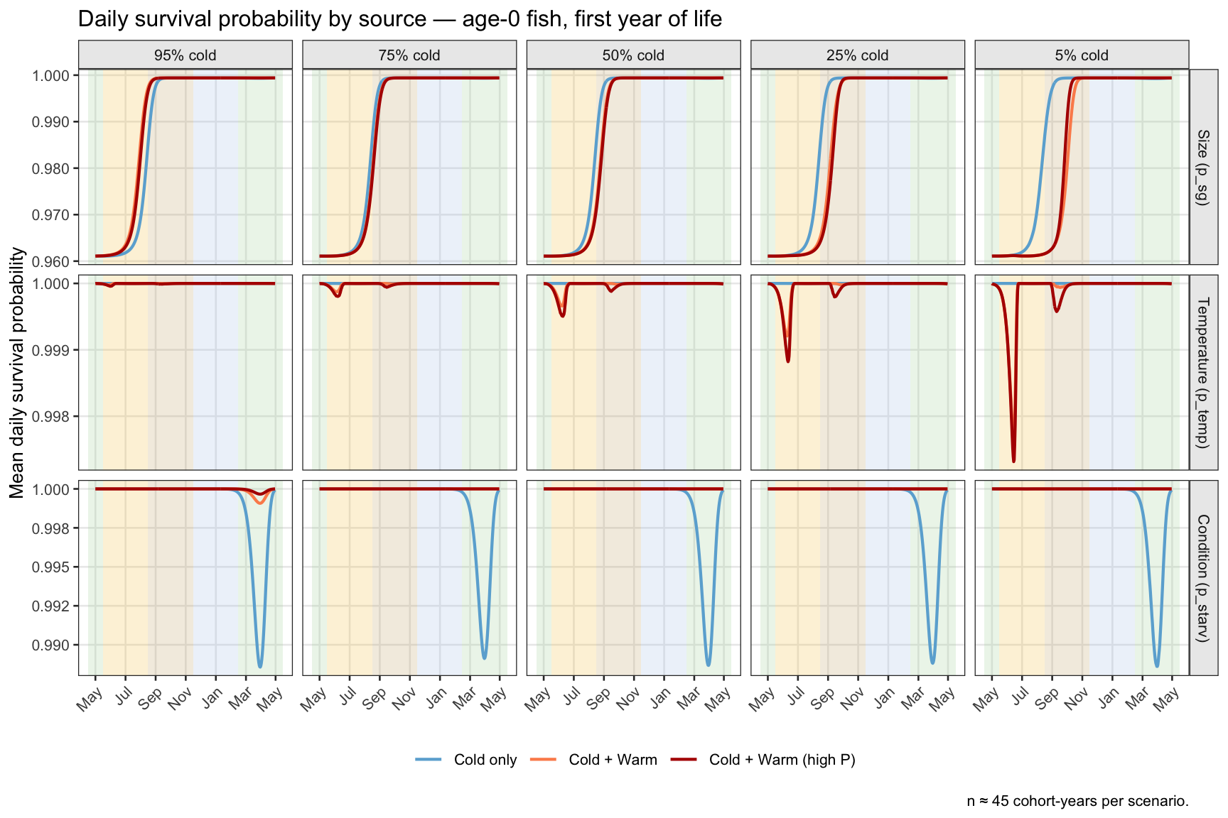
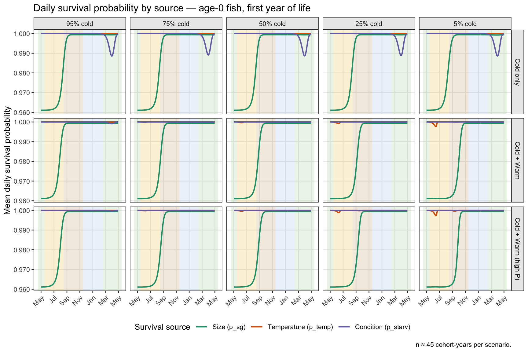
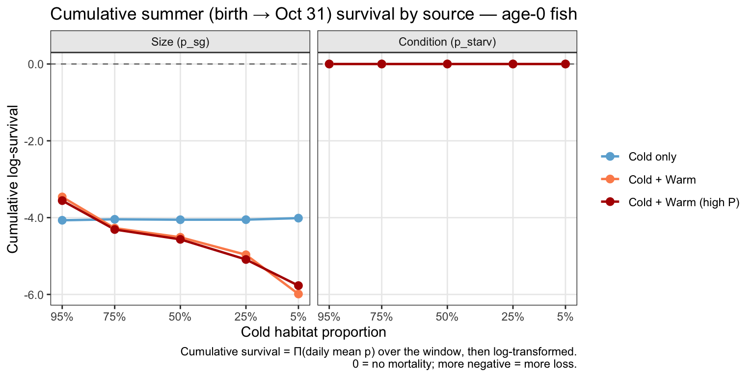
Because growth is stunted due to density dependence, age-0 summer survival rates are lower in the cold+warm scenarios compared to the cold-only scenarios, particularly as the cold patch shrinks.
First show mean daily survival probability by source tracked through the first year of life (day since hatch 0–364) for age-0 fish, averaged across all surviving fish and experimental-period cohort-years. Four components are shown: size-based ($p_{sg}$), temperature-based ($p_{temp}$), condition-based ($p_{starv}$), and age/senescence ($p_{age}$). Two facet layouts are provided for different comparative emphases.
```{r surv-daily-data}
#| cache: true
# f_surv_daily: mean daily survival probability by source for age-0 fish.
# Reuses p_sg_prob() defined above; fncSurvive* from Functions.qmd.
f_surv_daily <- function(df, exp_start) {
  df |>
    filter(age < 1, survived == 1, date >= exp_start) |>
    mutate(
      dsh     = as.integer(dayofsim - birth_dayofsim),
      p_sg    = fncSurviveSize(weight, minprob = base_params$s_min, maxprob = base_params$S_max_warm,
                               w0 = base_params$s_w0, k = base_params$s_k)[[1]],
      p_temp  = fncSurviveTemp(temp,      T1 = base_params$T1_mort,   T9 = base_params$T9_mort),
      p_starv = fncSurviveStarve(condition, K9 = base_params$K9_starv, K1 = base_params$K1_starv),
      p_age   = fncSurviveAge(age, x0 = 14, k = 0.7, p_min = 0.99)
    ) |>
    group_by(dsh) |>
    summarise(across(c(p_sg, p_temp, p_starv, p_age),
                     \(x) mean(x, na.rm = TRUE),
                     .names = "mean_{.col}"),
              n_fish = n(),
              .groups = "drop")
}

# All 15 scenarios; ibm_list_mech defined in the Mechanistic drivers setup chunk
surv_daily_raw <- lapply(ibm_list_mech, \(s) {
  f_surv_daily(s$df, exp_start_date) |>
    mutate(prop_cold = s$pc,
           hab_type  = s$ht,
           label     = scen_meta$label[scen_meta$prop_cold == s$pc])
})

surv_daily_df <- bind_rows(surv_daily_raw) |>
  mutate(
    label    = factor(label, levels = scen_meta$label),
    hab_type = factor(hab_type,
                      levels = c("Cold only", "Cold + Warm", "Cold + Warm (high P)"))
  ) |>
  pivot_longer(cols      = starts_with("mean_p_"),
               names_to  = "component",
               values_to = "mean_p",
               names_prefix = "mean_p_") |>
  mutate(component = factor(component,
    levels = c("sg",   "temp",                "starv",               "age"),
    labels = c("Size (p_sg)", "Temperature (p_temp)",
               "Condition (p_starv)", "Age (p_age)")))
```
Version 1: survival source in rows, cold proportion in columns, scenario as colour. *Note the longer period of low summer size-based survival in the cold+warm relative to cold-only scenarios, particularly as the cold patch shrinks*
```{r surv-daily-plot1}
#| fig-width: 9
#| fig-height: 6
dsh_brks <- c(0, 61, 122, 183, 244, 305, 365)
dsh_labs <- c("May","Jul","Sep","Nov","Jan","Mar","May")

# Seasonal bands on a daily (dsh) x-axis.
# Season boundaries from make_season_layers() are in msb units (months since
# April birth); multiply by 365/12 to convert to days since hatch.
# ymin/ymax span all survival probability rows; facet clipping handles the rest.
make_season_layers_dsh <- function(n_years = 1L, ymin = -Inf, ymax = Inf) {
  # Season boundaries converted from msb to dsh (days since hatch).
  # 1 msb = 365/12 ≈ 30.44 days. Default ymin/ymax = -Inf/Inf: fills each
  # panel's full height regardless of free y-scale (works on linear axes only;
  # log axes require finite bounds — use make_season_layers() instead).
  dpm       <- 365 / 12
  xmin_tmpl <- (c( 0.5,  1.5,  4.5,  7.5, 10.5)-1) * dpm
  xmax_tmpl <- (c( 1.5,  4.5,  7.5, 10.5, 13.5)-1) * dpm
  fill_tmpl <- c("#A8D5A2", "#F5C543", "#C8A96E", "#AEC6E8", "#A8D5A2")
  unlist(lapply(0:(n_years - 1L), \(y)
    lapply(seq_along(fill_tmpl), \(i)
      annotate("rect",
               xmin  = xmin_tmpl[i] + y * 365,
               xmax  = xmax_tmpl[i] + y * 365,
               ymin  = ymin, ymax = ymax,
               fill  = fill_tmpl[i],
               alpha = 0.22)
    )
  ), recursive = FALSE)
}

ggplot(filter(surv_daily_df, component != "Age (p_age)"),
       aes(x = dsh, y = mean_p, color = hab_type, group = hab_type)) +
  make_season_layers_dsh(1L) +
  geom_line(linewidth = 0.75) +
  facet_grid(component ~ label, scales = "free_y") +
  scale_color_manual(values = hab_cols, name = NULL) +
  scale_x_continuous(breaks = dsh_brks, labels = dsh_labs, minor_breaks = NULL) +
  scale_y_continuous(labels = scales::label_number(accuracy = 0.001)) +
  labs(
    x       = NULL,
    y       = "Mean daily survival probability",
    title   = "Daily survival probability by source \u2014 age-0 fish, first year of life",
    caption = "n \u2248 45 cohort-years per scenario."
  ) +
  theme_bw(base_size = 10) +
  theme(panel.grid.minor    = element_blank(),
        strip.background    = element_rect(fill = "grey92"),
        axis.text.x         = element_text(size = 8, angle = 45, hjust = 1),
        legend.position     = "bottom")
```
Version 2: scenario set in rows, cold proportion in columns, survival source as colour.
y-axis clipped to $[0.955,\, 1.001]$ to reveal within-panel structure across all four
components simultaneously.
```{r surv-daily-plot2}
#| fig-width: 9
#| fig-height: 6
mycols <- brewer.pal(3, "Dark2")
comp_cols_surv <- c(
  "Size (p_sg)"          = mycols[1],
  "Temperature (p_temp)" = mycols[2],
  "Condition (p_starv)"  = mycols[3]
)

ggplot(surv_daily_df %>% filter(component != "Age (p_age)"),
       aes(x = dsh, y = mean_p, color = component, group = component)) +
  make_season_layers_dsh(1L) +
  geom_line(linewidth = 0.75) +
  facet_grid(hab_type ~ label) +
  scale_color_manual(values = comp_cols_surv, name = "Survival source") +
  scale_x_continuous(breaks = dsh_brks, labels = dsh_labs, minor_breaks = NULL) +
  scale_y_continuous(labels = scales::label_number(accuracy = 0.001)) +
  # coord_cartesian(ylim = c(0.955, 1.001)) +
  labs(
    x       = NULL,
    y       = "Mean daily survival probability",
    title   = "Daily survival probability by source \u2014 age-0 fish, first year of life",
    caption = "n \u2248 45 cohort-years per scenario."
  ) +
  theme_bw(base_size = 10) +
  theme(panel.grid.minor    = element_blank(),
        strip.background    = element_rect(fill = "grey92"),
        axis.text.x         = element_text(size = 8, angle = 45, hjust = 1),
        legend.position     = "bottom")
```
By calculating cumulative log-survival (product of daily mean $p$) over the entire "summer" (birth to Oct 31) by source, we can see that size-based survival (due to density dependent effects on growth) dominates, with increasing survival costs as the cold patch shrinks, but only for cold+warm scenarios with elevated fry production
```{r surv-cum-plot}
#| fig-width: 8
#| fig-height: 4
# Computed from surv_daily_df (surv-daily-data chunk)
cum_surv_df <- surv_daily_df |>
  filter(component %in% c("Size (p_sg)", "Condition (p_starv)")) |>
  group_by(label, prop_cold, hab_type, component) |>
  summarise(
    summer = prod(mean_p[dsh <  183L]),
    winter = prod(mean_p[dsh >= 183L]),
    .groups = "drop"
  ) |>
  pivot_longer(c(summer, winter),
               names_to  = "season",
               values_to = "cum_surv") |>
  mutate(
    log_loss = log(cum_surv),
    season   = factor(season,
                      levels = c("summer", "winter"),
                      labels = c("Summer (birth \u2192 Nov)",
                                 "Winter (Nov \u2192 May)"))
  )

ggplot(cum_surv_df %>% filter(season == "Summer (birth \u2192 Nov)"),
       aes(x = prop_cold, y = log_loss,
           color = hab_type, shape = hab_type, group = hab_type)) +
  geom_hline(yintercept = 0, linewidth = 0.4, color = "grey40", linetype = "dashed") +
  geom_line(linewidth = 0.85) +
  geom_point(size = 2.8, shape = 16) +
  facet_wrap(~component, nrow = 1) +
  scale_color_manual(values = hab_cols, name = NULL) +
  scale_x_continuous(breaks = c(0.05, 0.25, 0.50, 0.75, 0.95),
                     labels = scales::label_percent(accuracy = 1),
                     transform = "reverse") +
  scale_y_continuous(labels = scales::label_number(accuracy = 0.1)) +
  labs(
    x       = "Cold habitat proportion",
    y       = "Cumulative log-survival",
    title   = "Cumulative summer (birth \u2192 Oct 31) survival by source \u2014 age-0 fish",
    caption = "Cumulative survival = \u03a0(daily mean p) over the window, then log-transformed.\n0 = no mortality; more negative = more loss."
  ) +
  theme_bw(base_size = 11) +
  theme(panel.grid.minor = element_blank(),
        strip.background = element_rect(fill = "grey92"),
        # axis.text.x      = element_text(angle = 45, hjust = 1),
        legend.position  = "right")
```
#### Fall "recruitment"
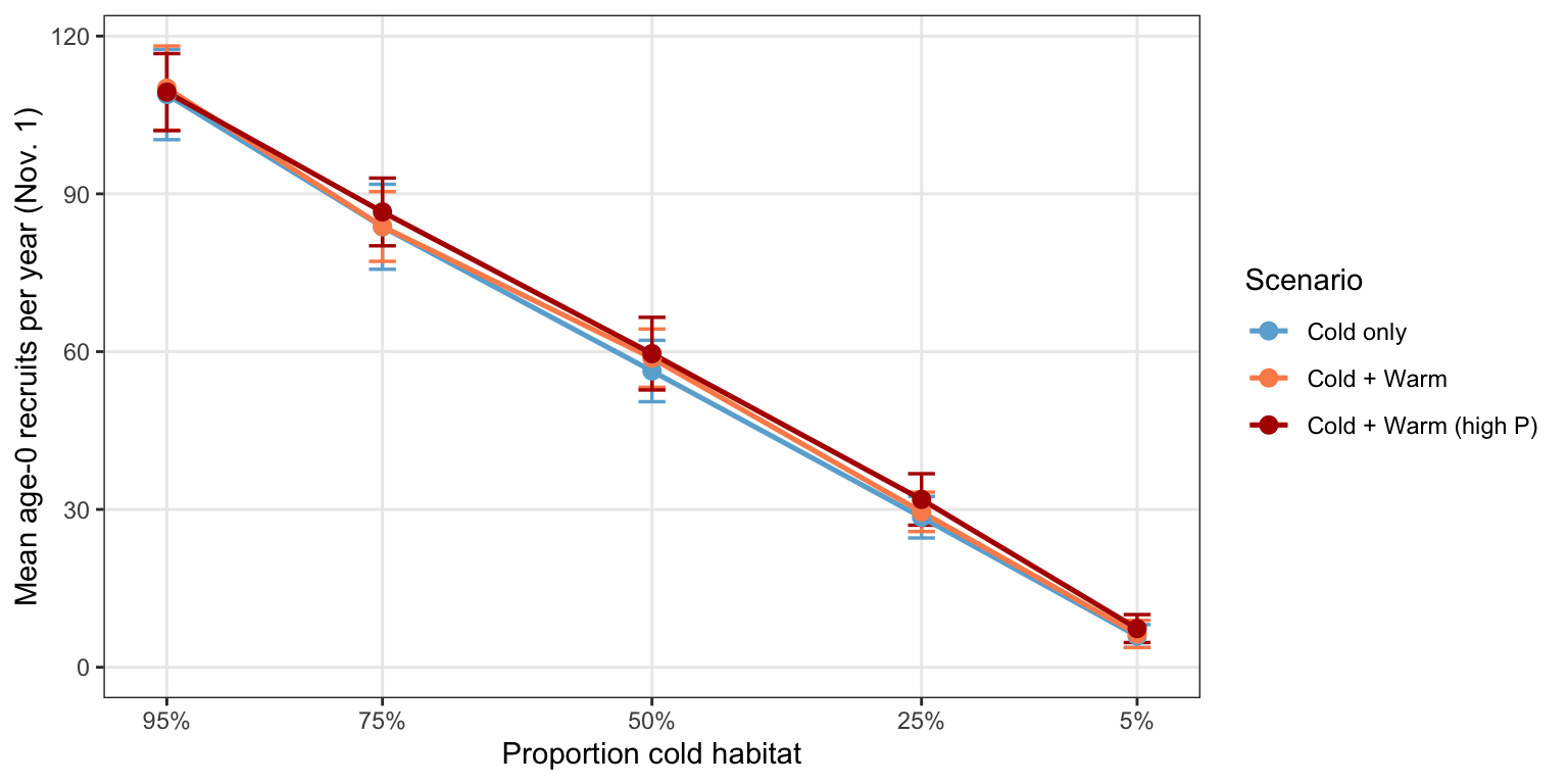
Collectively, this creates a substantial early life bottleneck, such that the number of surviving to the end of the first summer is purely a function of cold habitat availability, despite substantial differences in initial fry production owing to the relative availability of warm habitat.
```{r}
#| cache: false
#| fig-width: 8
#| fig-height: 4
mk_panel(full_df,
  mean_n_age0, pmax(mean_n_age0 - sd_n_age0, 0), mean_n_age0 + sd_n_age0,
  "Mean age-0 recruits per year (Nov. 1)", NULL, show_x = TRUE)
```
### Warm habitat availability mitigates winter losses
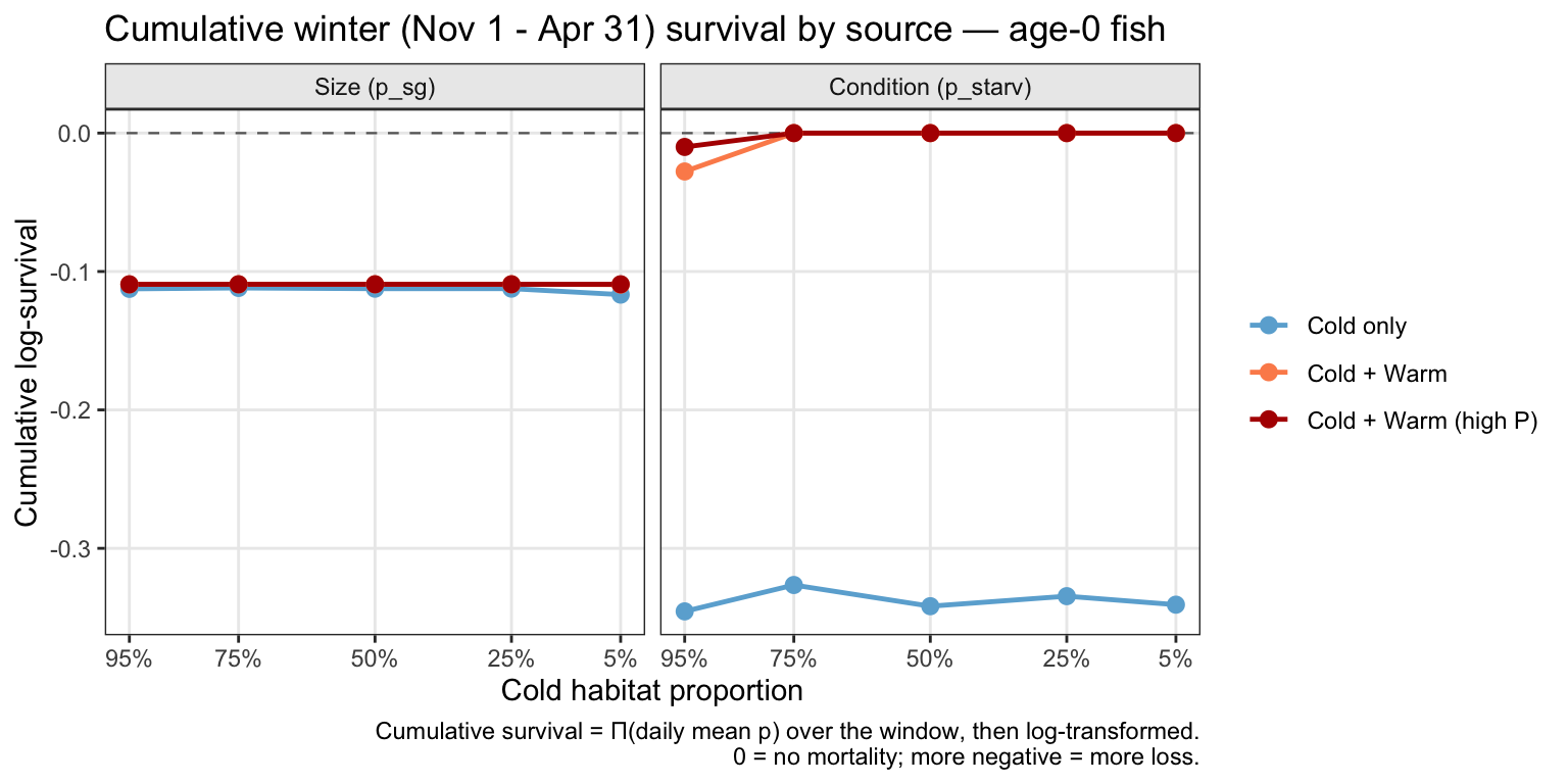
After November 1, all scenario classes enter their first winter with effectively the same number of age-0 fish — a direct consequence of cold habitat constraining summer recruitment. From this common baseline, the cold-only and cold+warm scenarios diverge sharply by the end of winter/early spring. The mechanism is condition-based (starvation) mortality: fish restricted to cold habitat cannot sustain adequate energy intake through winter, losing body mass until condition drops below the threshold that drives survival penalties. Fish with access to warm habitat can and do use it for continued foraging, (mostly) maintaining mass and avoiding further declines in abundance almost entirely.
#### Habitat use
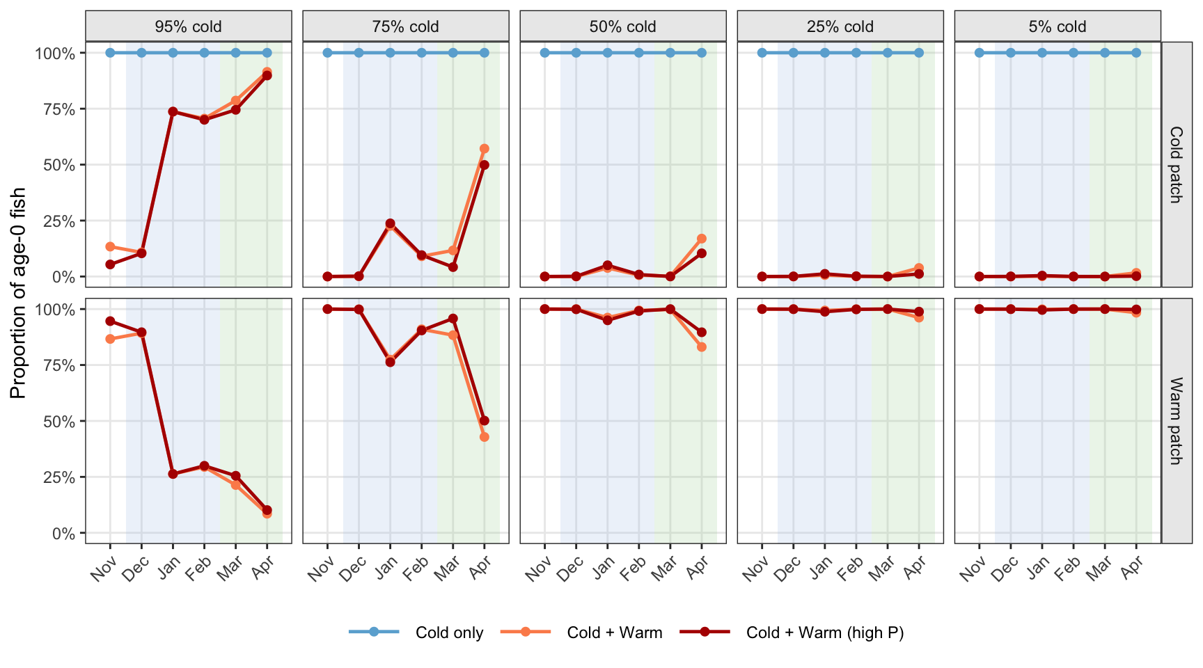
Fish move from cold to warm in the late fall (Oct-Nov). As cold proportion declines and warm increases, fish are more likely to remain in warm through the winter.
```{r hab-use-winter-prop}
#| fig-width: 9
#| fig-height: 5
ggplot(hab_use_age0 |> filter(msb > 6L),
       aes(x = msb, y = mean_prop, color = hab_type, group = hab_type)) +
  make_season_layers(4L, ymin = -Inf, ymax = Inf) +
  geom_line(linewidth = 0.85) +
  geom_point(size = 1.8) +
  facet_grid(patch_lab ~ label) +
  scale_color_manual(values = hab_cols, name = NULL) +
  scale_x_continuous(breaks = 7:12, labels = month.abb[c(11:12,1:4)],
                     minor_breaks = NULL, limits = c(6.5, 12.5)) +
  scale_y_continuous(limits = c(0, 1),
                     labels = scales::label_percent(accuracy = 1)) +
  labs(x = NULL, y = "Proportion of age-0 fish") +
  theme_bw(base_size = 11) +
  theme(panel.grid.minor   = element_blank(),
        strip.background   = element_rect(fill = "grey92"),
        axis.text.x        = element_text(size = 9, angle = 45, hjust = 1),
        legend.position    = "bottom",
        legend.key.width   = unit(1.2, "cm"))
```
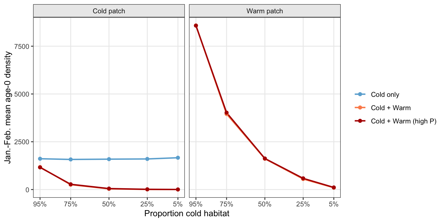
In summary, fish are preferrentially using the warm patch during winter, regardless of cold proportion. Winter densities are greater in the warm patch than in the cold patch, but this difference shrinks as the proportion of cold habitat declines (largely mediated by area).
```{r}
#| fig-width: 8
#| fig-height: 4
hab_use_age0 |> filter(msb %in% c(9:10)) |> group_by(prop_cold, hab_type, label, patch_lab) |> summarise(mean_density = mean(mean_density)) |> ungroup() |>
  ggplot(aes(x = prop_cold, y = mean_density, color = hab_type, group = hab_type)) +
  geom_line(linewidth = 0.85) +
  geom_point(size = 1.8) +
  facet_wrap(~patch_lab, nrow = 1) +
  scale_color_manual(values = hab_cols, name = NULL) +
  scale_x_reverse(breaks = pc_levels,
                  labels = scales::percent_format(accuracy = 1)) +
  # scale_y_continuous(limits = c(0, 1),
  #                    labels = scales::label_number(accuracy = 0.1)) +
  labs(x = "Proportion cold habitat", y = "Jan.-Feb. mean age-0 density") +
  theme_bw(base_size = 11) +
  theme(panel.grid.minor   = element_blank(),
        strip.background   = element_rect(fill = "grey92"),
        # axis.text.x        = element_text(size = 9, angle = 45, hjust = 1),
        legend.position    = "right")
```
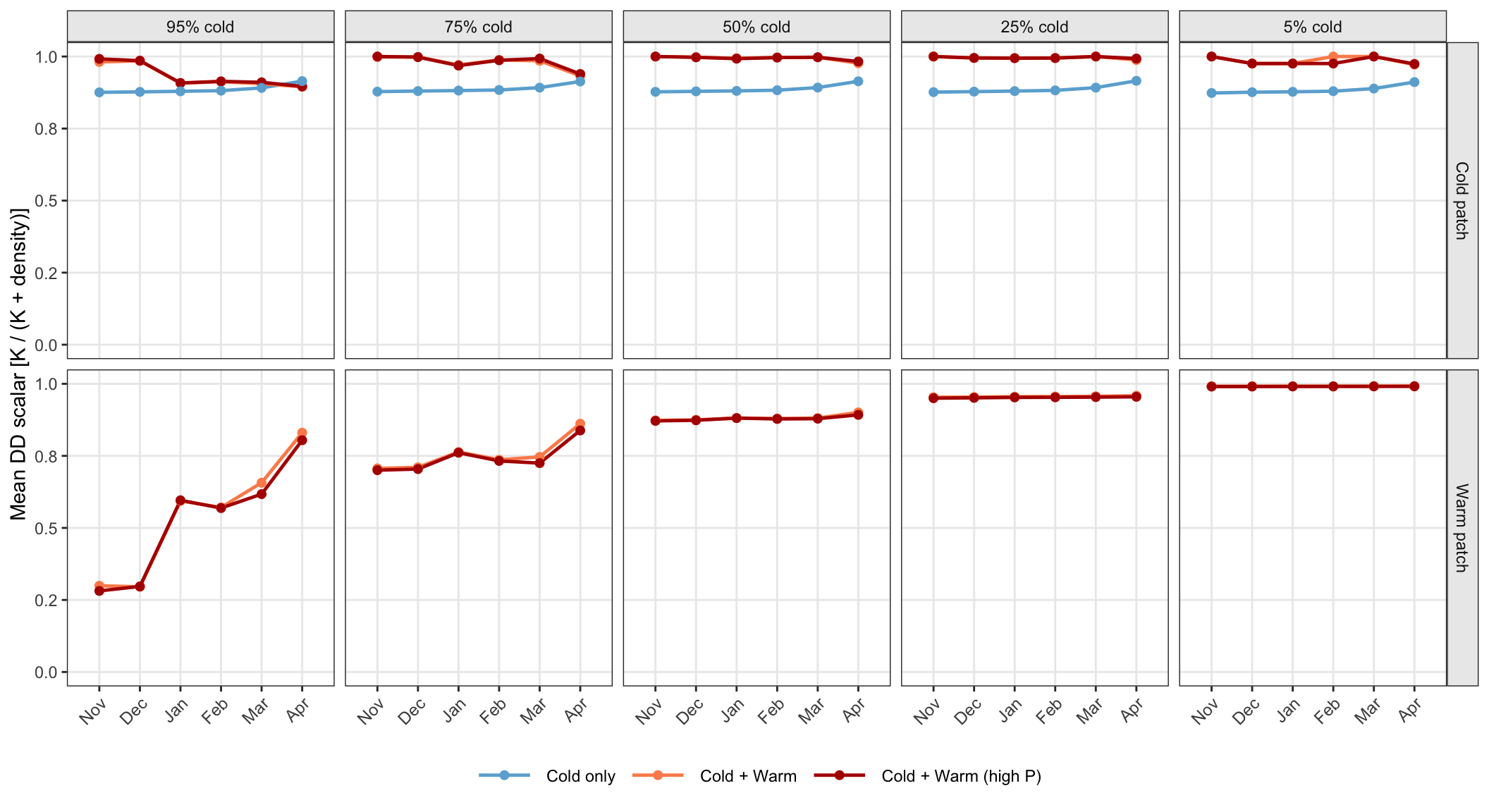
#### Density dependence
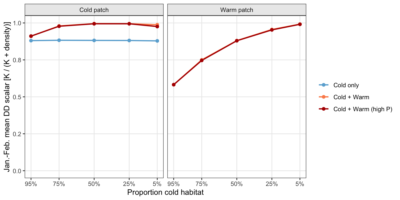
Fish are basically ~input matching: when warm habitat is rare, higher densities mean increased strength of density dependence (lower DD scalar) in warm. Cold patch DD is stronger for cold-only scenarios relative to cold-warm, because all fish are forced to use cold habitat during winter, while fish in cold+warm scenarios can disperse to warm habitat.
```{r dd-winter-plot}
#| fig-width: 11
#| fig-height: 6
ggplot(dd_age0_df |> filter(msb > 6L),
       aes(x = msb, y = mean_dd, color = hab_type, group = hab_type)) +
  # make_season_layers(1L, ymin = 0, ymax = 1) +
  geom_line(linewidth = 0.85) +
  geom_point(size = 1.8) +
  facet_grid(patch_lab ~ label) +
  scale_color_manual(values = hab_cols, name = NULL) +
  scale_x_continuous(breaks = 7:12, labels = month.abb[c(11:12,1:4)],
                     minor_breaks = NULL, limits = c(6.5, 12.5)) +
  scale_y_continuous(limits = c(0, 1),
                     labels = scales::label_number(accuracy = 0.1)) +
  labs(x = NULL, y = "Mean DD scalar [K / (K + density)]") +
  theme_bw(base_size = 11) +
  theme(panel.grid.minor   = element_blank(),
        strip.background   = element_rect(fill = "grey92"),
        axis.text.x        = element_text(size = 9, angle = 45, hjust = 1),
        legend.position    = "bottom",
        legend.key.width   = unit(1.2, "cm"))
```
```{r}
#| fig-width: 8
#| fig-height: 4
#|
dd_age0_df |> filter(msb %in% c(9:10)) |> group_by(prop_cold, hab_type, label, patch_lab) |> summarise(mean_dd = mean(mean_dd)) |> ungroup() |>
  ggplot(aes(x = prop_cold, y = mean_dd, color = hab_type, group = hab_type)) +
  geom_line(linewidth = 0.85) +
  geom_point(size = 1.8) +
  facet_wrap(~patch_lab, nrow = 1) +
  scale_color_manual(values = hab_cols, name = NULL) +
  scale_x_reverse(breaks = pc_levels,
                  labels = scales::percent_format(accuracy = 1)) +
  scale_y_continuous(limits = c(0, 1),
                     labels = scales::label_number(accuracy = 0.1)) +
  labs(x = "Proportion cold habitat", y = "Jan.-Feb. mean DD scalar [K / (K + density)]") +
  theme_bw(base_size = 11) +
  theme(panel.grid.minor   = element_blank(),
        strip.background   = element_rect(fill = "grey92"),
        # axis.text.x        = element_text(size = 9, angle = 45, hjust = 1),
        legend.position    = "right")
```
#### Consumption
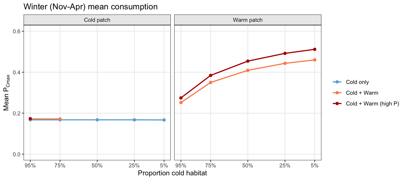
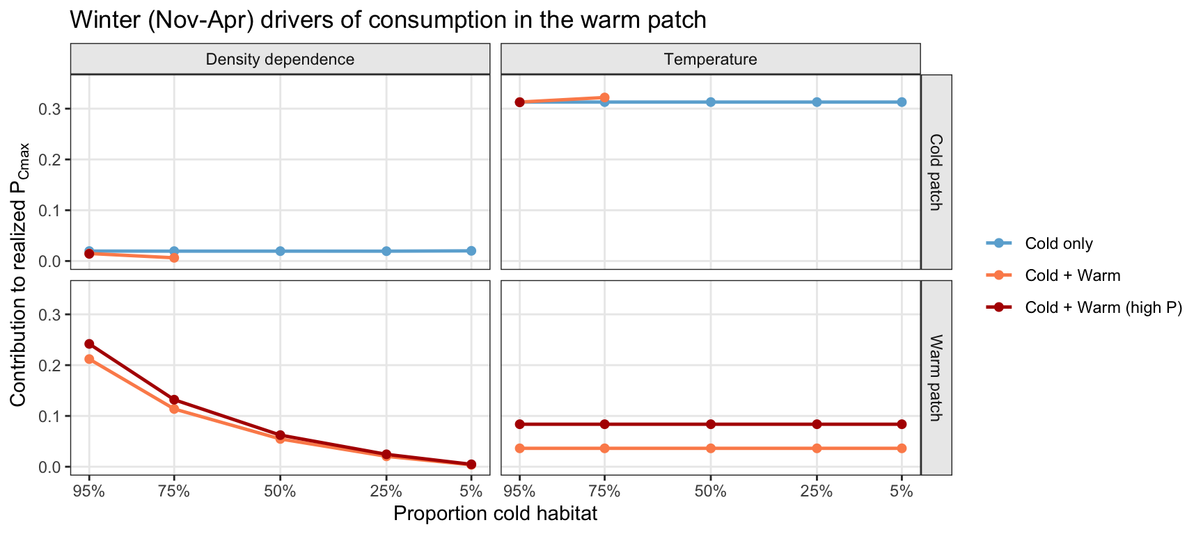
During winter, consumption is entirely constrained by cold patch temperature in the cold-only scenarios. In contrast, temperature and density dependence in the warm patch combine to constrain consumption in the cold+warm scenarios. When proportion cold is high (warm habitat is rare), density dependence in the warm habitat is primarily limiting consumption. But when proportion cold is low (warm habitat is abundant), density dependence in the warm habitat is less significant, and temperature becomes the primary constraint. As a result, cold+warm fish feed at higher rates than cold-only fish, and cold+warm consumption increases as cold habitat is increasingly replaced by warm habitat.
```{r}
#| fig-width: 11
#| fig-height: 7
# Decomposition of realized p-value into temperature and density-dependence
# components across the full age-0 year, for both cold and warm patches.
#   Dashed line  = mean_pcmax_adj  (temperature ceiling; DD removed)
#   Solid line   = mean_realized_p (after DD suppression)
#   Shaded gap   = density-dependence suppression alone
# Cold patch: DD gap widens in early summer for cold+warm scenarios (more fish
#   from warm-enabled reproduction flooding into cold habitat).
# Warm patch: temperature ceiling collapses near peak summer (~Jul–Aug) as
#   fncTempDepend approaches 0 near 24°C, independently of density. Cold-only
#   scenarios have no warm patch and are absent from the bottom row.
# Per-patch, per-hab_type pcmax baseline reference lines.
# Cold patch: single dotted line at 0.5 (same for all scenarios).
# Warm patch: color-coded dotted lines at 0.5 (Cold + Warm) and 0.6 (high P).
pcmax_refs <- data.frame(
  patch_lab  = c("Cold patch", "Warm patch",   "Warm patch"),
  hab_type   = c(NA_character_, "Cold + Warm", "Cold + Warm (high P)"),
  pcmax_base = c(0.5,           0.5,            0.6)
)

pcmax_age0_df |>
  ggplot(aes(x = msb, color = hab_type, fill = hab_type, group = hab_type)) +
  geom_hline(data = pcmax_refs |> filter(is.na(hab_type)),
             aes(yintercept = pcmax_base), inherit.aes = FALSE,
             color = "grey70", linetype = "dotted", linewidth = 0.4) +
  geom_segment(data = pcmax_refs |> filter(!is.na(hab_type)),
               aes(x = 0.5, xend = 12.5,
                   y = pcmax_base, yend = pcmax_base, color = hab_type),
               inherit.aes = FALSE,
               linetype = "dotted", linewidth = 0.4) +
  geom_ribbon(aes(ymin = mean_realized_p, ymax = mean_pcmax_adj),
              alpha = 0.18, color = NA) +
  geom_line(aes(y = mean_pcmax_adj), linetype = "dashed", linewidth = 0.65) +
  geom_line(aes(y = mean_realized_p), linewidth = 0.85) +
  facet_grid(patch_lab ~ label) +
  scale_color_manual(values = hab_cols, name = NULL) +
  scale_fill_manual(values  = hab_cols, name = NULL, breaks = names(hab_cols)) +
  scale_x_continuous(breaks = 1:12, labels = age0_msb_labs, minor_breaks = NULL) +
  scale_y_continuous(limits = c(0, 0.65),
                     labels = scales::label_number(accuracy = 0.1)) +
  labs(x = NULL,
       y = "p-value (proportion of max consumption)",
       caption = "Solid = realized p  |  Dashed = temperature ceiling  |  Shaded gap = density-dependence suppression  |  Dotted = pcmax baseline") +
  theme_bw(base_size = 11) +
  theme(panel.grid.minor   = element_blank(),
        strip.background   = element_rect(fill = "grey92"),
        axis.text.x        = element_text(size = 8, angle = 45, hjust = 1),
        legend.position    = "bottom",
        legend.key.width   = unit(1.2, "cm"))
```
```{r}
#| fig-width: 9
#| fig-height: 4
#|
pcmax_age0_df %>%
  mutate(season = ifelse(msb %in% c(1:6), "summer", "winter")#,
         # dd_gap = replace_na(dd_gap, 0),
         # temp_gap = replace_na(temp_gap, 0)
         ) %>%
  filter(season == "winter") %>%
  group_by(prop_cold, hab_type, patch_lab, season) %>%
  summarize(mean_realized_p = mean(mean_realized_p)) %>%
  ungroup() %>%
  ggplot(aes(x = prop_cold, y = mean_realized_p, group = hab_type, color = hab_type)) +
  geom_line(linewidth = 0.85) +
  geom_point(size = 1.8) +
  facet_wrap(~patch_lab) +
  scale_color_manual(values = hab_cols, name = NULL) +
  scale_x_reverse(breaks = pc_levels,
                  labels = scales::percent_format(accuracy = 1)) +
    scale_y_continuous(limits = c(0, 0.6)) +
  labs(x = "Proportion cold habitat", y = expression(Mean~P[Cmax]),
       title = "Winter (Nov-Apr) mean consumption") +
  theme_bw(base_size = 11) +
  theme(panel.grid.minor   = element_blank(),
        strip.background   = element_rect(fill = "grey92"),
        # axis.text.x        = element_text(size = 9, angle = 45, hjust = 1),
        legend.position    = "right")
pcmax_age0_df %>%
  mutate(season = ifelse(msb %in% c(1:6), "summer", "winter")#,
         # dd_gap = replace_na(dd_gap, 0),
         # temp_gap = replace_na(temp_gap, 0)
         ) %>%
  group_by(prop_cold, hab_type, patch_lab, season) %>%
  summarize(mean_dd_gap = mean(dd_gap),
            mean_temp_gap = mean(temp_gap)) %>%
  ungroup() %>%
  filter(season == "winter") %>%
  gather(mean_dd_gap:mean_temp_gap, key = "driver", value = "mean_gap") %>%
  mutate(driver = recode(driver, "mean_dd_gap" = "Density dependence", "mean_temp_gap" = "Temperature")) %>%
  ggplot(aes(x = prop_cold, y = mean_gap, group = hab_type, color = hab_type)) +
  geom_line(linewidth = 0.85) +
  geom_point(size = 1.8) +
  facet_grid(patch_lab~driver) +
  scale_color_manual(values = hab_cols, name = NULL) +
  scale_x_reverse(breaks = pc_levels,
                  labels = scales::percent_format(accuracy = 1)) +
    scale_y_continuous(limits = c(0, 0.35)) +
  labs(x = "Proportion cold habitat", y = expression(Contribution~to~realized~P[Cmax]),
       title = "Winter (Nov-Apr) drivers of consumption in the warm patch") +
  theme_bw(base_size = 11) +
  theme(panel.grid.minor   = element_blank(),
        strip.background   = element_rect(fill = "grey92"),
        # axis.text.x        = element_text(size = 9, angle = 45, hjust = 1),
        legend.position    = "right")
```
#### Growth
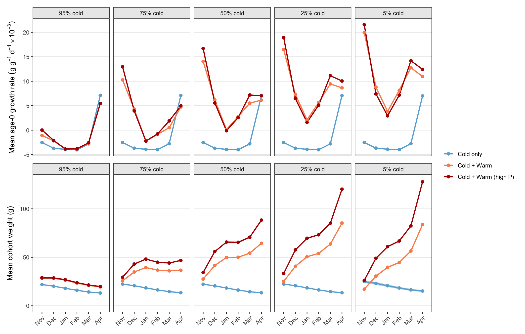
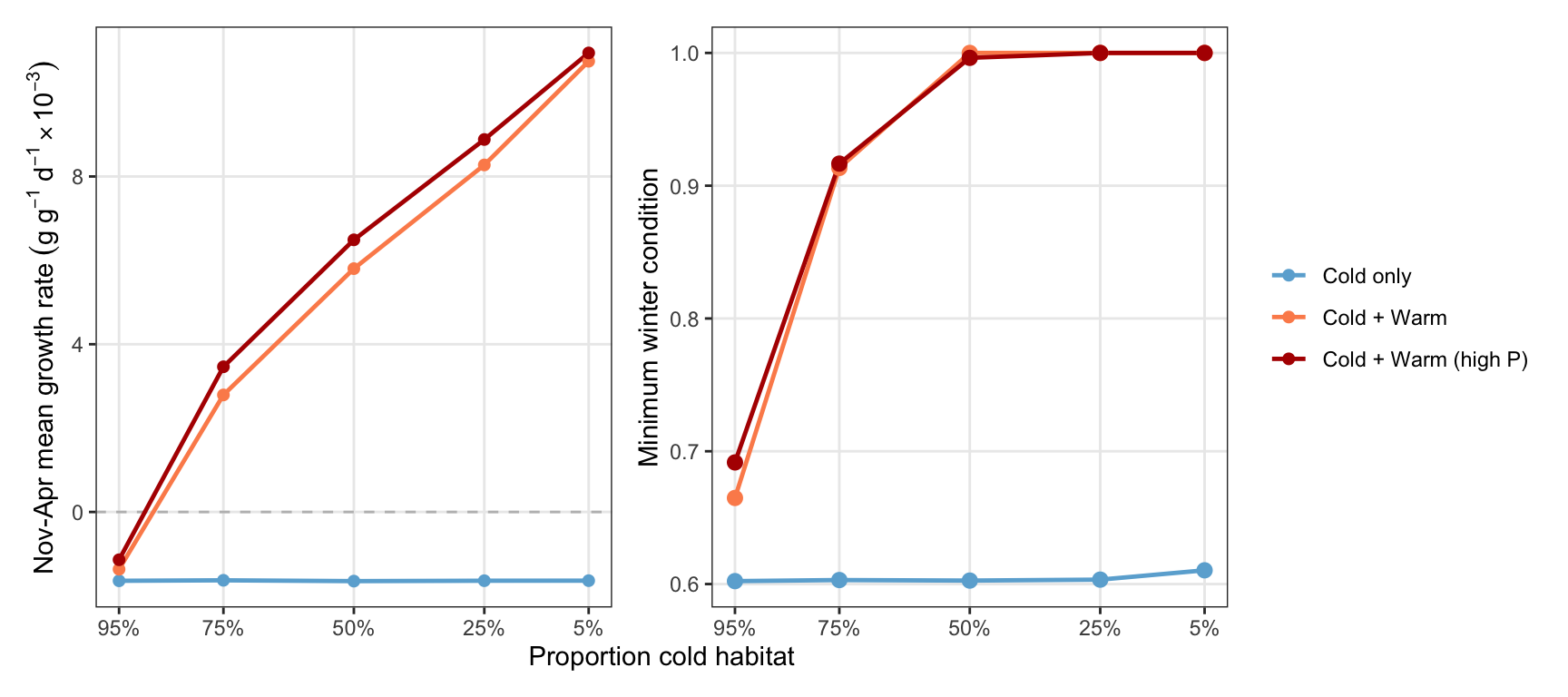
Cold-only fish thus experience consistently negative growth rates overwinter, leading to reduce condition across all cold proportions. In contrast, mean winter growth rates for cold-warm fish increase as warm habitat becomes more available (declining density dependent constraints on consumption), and fish are better able to avoid declines in condition.
```{r gr-size-winter-plot}
#| fig-width: 11
#| fig-height: 7
summer_msb_labs <- month.abb[c(11:12,1:4)]

# ── A: Monthly age-0 growth rate trajectories, Nov-Apr ───────────────────────
pA_sgr <- ggplot(gr_age0_df |> filter(msb > 6L),
                 aes(x = msb, y = mean_ggd,
                     color = hab_type, group = hab_type)) +
  # make_season_layers(1L, ymin = -10, ymax = 40) +
  # geom_hline(yintercept = 0, linetype = "dashed", color = "grey50", linewidth = 0.45) +
  geom_line(linewidth = 0.85) +
  geom_point(size = 1.8) +
  facet_wrap(~ label, nrow = 1) +
  scale_color_manual(values = hab_cols, name = NULL) +
  scale_x_continuous(breaks = 7:12, labels = summer_msb_labs,
                     minor_breaks = NULL, limits = c(6.5, 12.5)) +
  labs(x = NULL,
       y = expression("Mean age-0 growth rate" ~ (g ~ g^{-1} ~ d^{-1} %*% 10^{-3}))) +
  theme_bw(base_size = 11) +
  theme(panel.grid.minor   = element_blank(),
        panel.grid.major.x = element_blank(),
        strip.background   = element_rect(fill = "grey92"),
        axis.text.x        = element_blank(),
        axis.ticks.x       = element_blank(),
        plot.tag           = element_text(face = "bold"),
        legend.position    = "right")

# ── B: Summer weight trajectories (msb 1–6, May through Oct) ─────────────────
pB_swt <- ggplot(wt_age0_df |> filter(msb > 6L),
                 aes(x = msb, y = wt_mean,
                     color = hab_type, group = hab_type)) +
  # make_season_layers(1L, ymin = 0, ymax = 200) +
  geom_ribbon(aes(ymin = pmax(0, wt_mean - 1.96 * wt_se),
                  ymax = wt_mean + 1.96 * wt_se,
                  fill = hab_type),
              alpha = 0.5, color = NA) +
  geom_line(linewidth = 0.85) +
  geom_point(size = 1.8) +
  # geom_hline(yintercept = base_params$s_w0, linetype = "dashed", color = "grey50", linewidth = 0.45) +
  facet_wrap(~ label, nrow = 1) +
  scale_color_manual(values = hab_cols, name = NULL) +
  scale_fill_manual(values  = hab_cols, name = NULL, breaks = names(hab_cols)) +
  scale_x_continuous(breaks = 7:12, labels = summer_msb_labs,
                     minor_breaks = NULL, limits = c(6.5, 12.5)) +
  scale_y_continuous(limits = c(0, NA)) +
  labs(x = NULL, y = "Mean cohort weight (g)") +
  theme_bw(base_size = 11) +
  theme(panel.grid.minor   = element_blank(),
        panel.grid.major.x = element_blank(),
        strip.background   = element_rect(fill = "grey92"),
        axis.text.x        = element_text(size = 9, angle = 45, hjust = 1),
        plot.tag           = element_text(face = "bold"),
        legend.position    = "none")

(pA_sgr / pB_swt) +
  plot_layout(guides = "collect", heights = c(1, 1))
```
```{r }
#| fig-width: 9
#| fig-height: 4
# mean May-Aug growth rates
pA_mgd <- gr_age0_df |> filter(msb %in% c(7:12)) |> group_by(prop_cold, hab_type, label) |> summarise(mean_ggd = mean(mean_ggd)) |> ungroup() |>
  ggplot(aes(x = prop_cold, y = mean_ggd, color = hab_type, group = hab_type)) +
  geom_hline(yintercept = 0, linetype = "dashed", color = "grey") +
  geom_line(linewidth = 0.85) +
  geom_point(size = 1.8) +
  # facet_wrap(~patch_lab, nrow = 1) +
  scale_color_manual(values = hab_cols, name = NULL) +
  scale_x_reverse(breaks = pc_levels,
                  labels = scales::percent_format(accuracy = 1)) +
  # scale_y_continuous(limits = c(0, 1),
  #                    labels = scales::label_number(accuracy = 0.1)) +
  labs(x = "Proportion cold habitat", y = expression("Nov-Apr mean growth rate" ~ (g ~ g^{-1} ~ d^{-1} %*% 10^{-3}))) +
  theme_bw(base_size = 11) +
  theme(panel.grid.minor   = element_blank(),
        strip.background   = element_rect(fill = "grey92"),
        # axis.text.x        = element_text(size = 9, angle = 45, hjust = 1),
        legend.position    = "right")

### condition
pB_mcond <- wt_age0_df %>%
  group_by(hab_type, label, prop_cold) %>%
  mutate(peak_wt = cummax(wt_mean)) %>%
  ungroup() %>%
  mutate(condition = wt_mean / peak_wt) %>%
  filter(msb %in% c(7:12)) %>%
  group_by(hab_type, label, prop_cold) %>%
  summarize(min_condition = min(condition)) %>%
  ungroup() %>%
  ggplot(aes(x = prop_cold, y = min_condition, color = hab_type, group = hab_type)) +
  geom_line(linewidth = 0.85) +
  geom_point(size = 2.5) +
  scale_color_manual(values = hab_cols, name = NULL) +
  scale_x_reverse(breaks = pc_levels,
                  labels = scales::percent_format(accuracy = 1)) +
  labs(x = "Proportion cold habitat",
       y = "Minimum winter condition") +
  theme_bw(base_size = 11) +
  theme(panel.grid.minor = element_blank(),
        legend.position  = "none")


(pA_mgd + pB_mcond) +
  plot_layout(guides = "collect", axes = "collect") +
  labs(x = "Proportion cold habitat")
```
#### Survival
```{r}
#| fig-width: 8
#| fig-height: 4
#|
ggplot(cum_surv_df %>% filter(season == "Winter (Nov \u2192 May)"),
       aes(x = prop_cold, y = log_loss,
           color = hab_type, shape = hab_type, group = hab_type)) +
  geom_hline(yintercept = 0, linewidth = 0.4, color = "grey40", linetype = "dashed") +
  geom_line(linewidth = 0.85) +
  geom_point(size = 2.8, shape = 16) +
  facet_wrap(~component, nrow = 1) +
  scale_color_manual(values = hab_cols, name = NULL) +
  scale_x_continuous(breaks = c(0.05, 0.25, 0.50, 0.75, 0.95),
                     labels = scales::label_percent(accuracy = 1),
                     transform = "reverse") +
  scale_y_continuous(labels = scales::label_number(accuracy = 0.1)) +
  labs(
    x       = "Cold habitat proportion",
    y       = "Cumulative log-survival",
    title   = "Cumulative winter (Nov 1 - Apr 31) survival by source \u2014 age-0 fish",
    caption = "Cumulative survival = \u03a0(daily mean p) over the window, then log-transformed.\n0 = no mortality; more negative = more loss."
  ) +
  theme_bw(base_size = 11) +
  theme(panel.grid.minor = element_blank(),
        strip.background = element_rect(fill = "grey92"),
        # axis.text.x      = element_text(angle = 45, hjust = 1),
        legend.position  = "right")
```
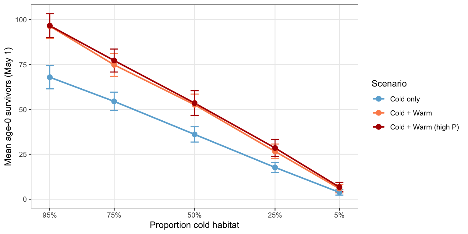
#### Spring "recruitment"
After the shared summer bottleneck sets a common Nov. 1 baseline, the cold-only and cold+warm scenarios diverge through winter. Cold-only fish face a second condition-driven mortality episode in late winter/early spring that warm-habitat fish largely avoid. By April 1 — the end of the first year of life — the scenarios separate clearly: cold+warm (and especially high-P) cohorts retain substantially more survivors than cold-only cohorts at equivalent cold proportions, and the divergence grows as warm habitat increases.
```{r}
#| cache: false
#| fig-width: 8
#| fig-height: 4
mk_panel(full_df,
  mean_n_apr1, pmax(mean_n_apr1 - sd_n_apr1, 0), mean_n_apr1 + sd_n_apr1,
  "Mean age-0 survivors (May 1)", NULL, show_x = TRUE)
```
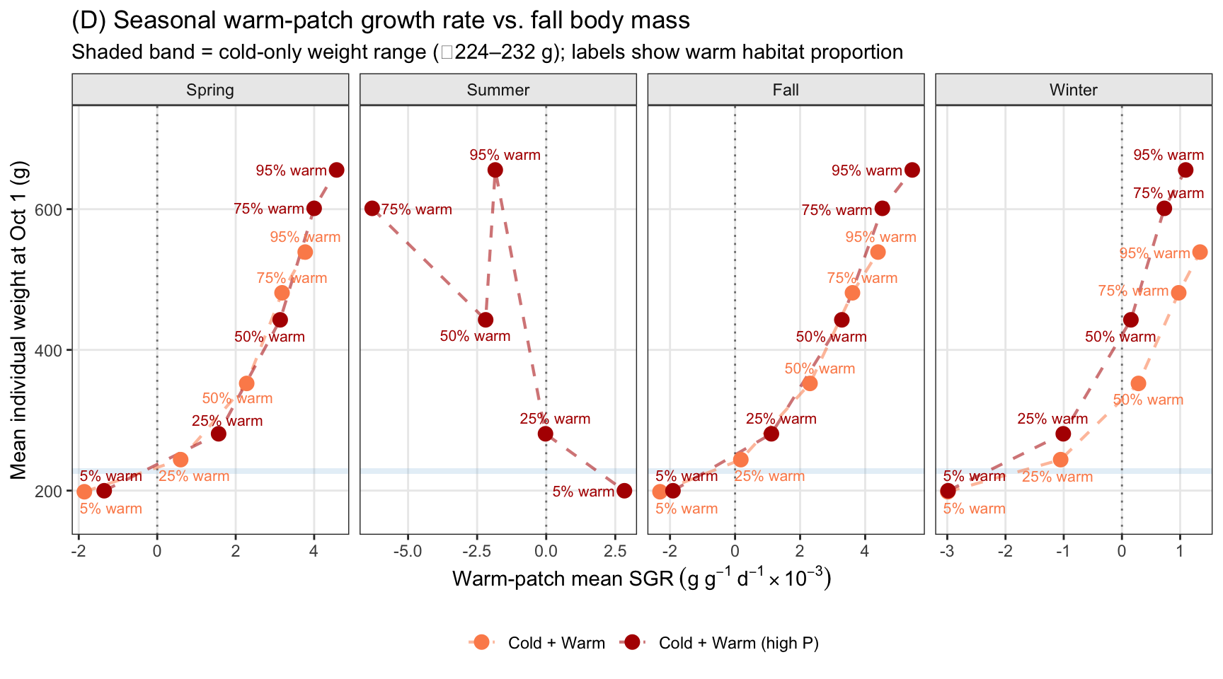
## Warm habitat and seasonal body-mass accumulation
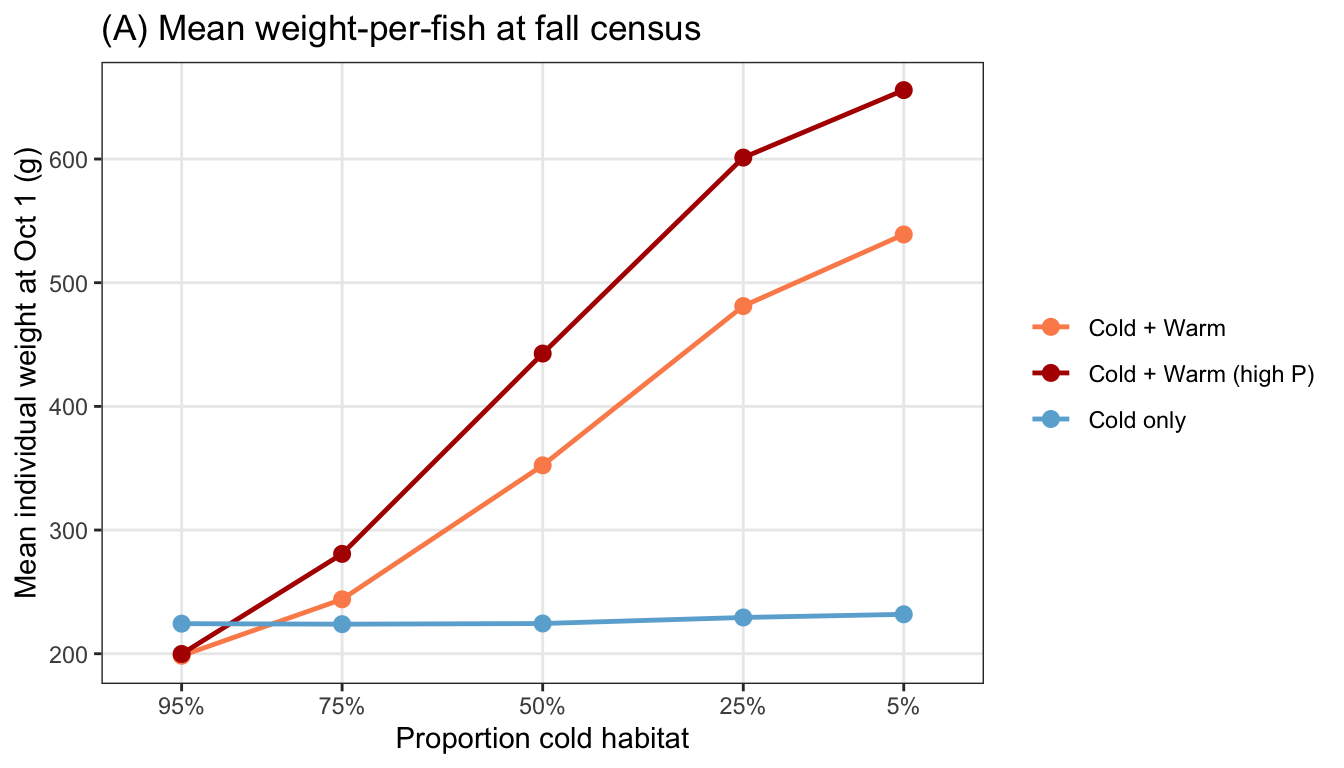
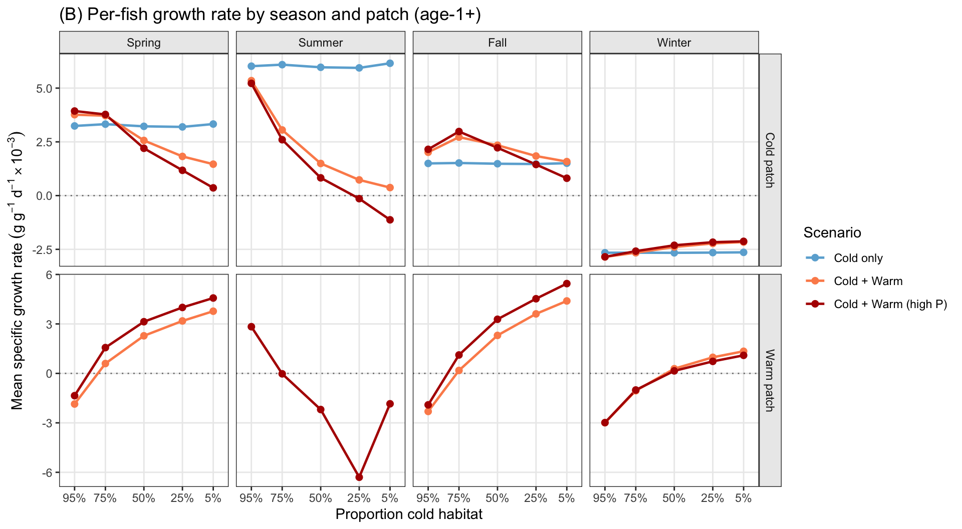
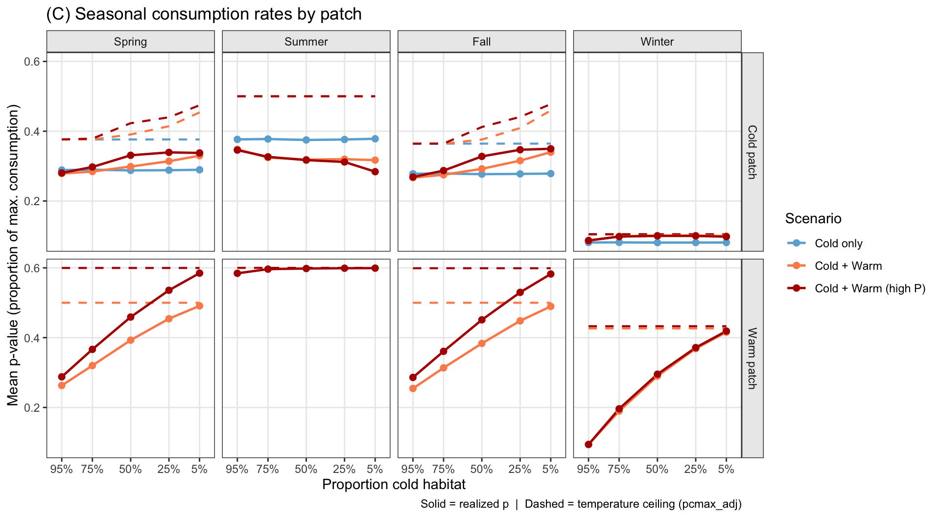
The preceding weight-at-age panels show that cold+warm fish are substantially heavier at a given age than cold-only fish, and the gap widens as warm habitat proportion grows. This section traces the weight-at-age difference mechanistically to supplemental growth opportunities provided by the warm patch — primarily in **fall (Sep–Nov)** and **spring (Mar–May)**, when warm-patch temperatures allow substantially higher consumption and growth rates than the cold patch.
**Figure summary:**
* **(A)** Mean individual body mass at Oct 1 — the end-point observation.
* **(B)** Per-fish specific growth rate by season and patch — warm-patch fish grow faster than cold-patch fish in fall and spring; the advantage scales with warm habitat availability and collapses when the warm patch is too small to relieve density dependence.
* **(C)** Seasonal consumption rates by patch — identifies the proximate mechanism: in fall and spring the warm patch sustains a substantially higher temperature ceiling and realized p-value than the cold patch; density-dependent suppression erodes the realized advantage as the warm patch shrinks.
* **(D)** Synthesis scatterplot — warm-patch fall and spring growth rates vs. Oct 1 body mass, directly quantifying the link between seasonal warm-patch growth opportunities and realized weight-at-age.
#### Data
```{r winter-bm-data}
#| cache: true
# Per-fish mean specific growth rate (ggd × 10⁻³ g/g/d) by season × patch.
# Averaged across all surviving fish and experimental-period years.
# Requires ibm_list_mech (defined in the Mechanistic drivers setup chunk).

compute_seasonal_ggd <- function(s) {
  s$df |>
    filter(date >= exp_start_date, survived == 1, !is.na(ggd), floor(age) >= 1) |>
    mutate(
      mo     = month(date),
      season = factor(
        case_when(
          mo %in% c(12,1,2)    ~ "Winter",
          mo %in% c(3:5)       ~ "Spring",
          mo %in% c(6:8)       ~ "Summer",
          mo %in% c(9:11)      ~ "Fall"
        ),
        levels = c("Spring", "Summer", "Fall", "Winter")
      )
    ) |>
    group_by(season, patch) |>
    summarise(mean_ggd = mean(ggd, na.rm = TRUE) * 1000, .groups = "drop") |>
    mutate(prop_cold = s$pc, hab_type = s$ht)
}

seasonal_ggd_df <- bind_rows(lapply(ibm_list_mech, compute_seasonal_ggd)) |>
  left_join(scen_meta, by = "prop_cold") |>
  mutate(
    label     = factor(label,    levels = scen_meta$label),
    hab_type  = factor(hab_type, levels = c("Cold only", "Cold + Warm", "Cold + Warm (high P)")),
    patch_lab = factor(
      if_else(patch == "warm", "Warm patch", "Cold patch"),
      levels = c("Cold patch", "Warm patch")
    )
  )
```
```{r seasonal-p-data}
#| cache: true
# Seasonal mean consumption-rate summaries by patch for ALL fish (not just age-0).
# Uses the same bioenergetics decomposition as pcmax_age0_df but applied to the
# full population on each simulated date:
#   temperature ceiling:  pcmax_adj  = min(fncTempDepend(temp), pcmax_baseline)
#   density-dep. scalar:  dd_scalar  = K / (K + n_fish_in_patch / patch_area)
#   realized p-value:     realized_p = pcmax_adj * dd_scalar
#
# pcmax baselines: cold patch = 0.5 (all scenarios);
#                  warm patch = 0.5 (Cold+Warm) or 0.6 (high P); NA (Cold only).
# Season definitions match winter-bm-data: Dec–Feb = Winter, Mar–May = Spring,
# Jun–Aug = Summer, Sep–Nov = Fall.

compute_seasonal_p_all <- function(s) {
  a_cold     <- s$pc * 2.0
  a_warm     <- (1 - s$pc) * 2.0
  K          <- base_params$K_cold
  pcmax_cold <- 0.5
  pcmax_warm <- switch(s$ht,
    "Cold + Warm"          = 0.5,
    "Cold + Warm (high P)" = 0.6,
    NA_real_
  )

  s$df |>
    filter(date >= exp_start_date, survived == 1, floor(age) >= 1) |>
    mutate(
      mo     = month(date),
      season = factor(
        case_when(
          mo %in% c(12L, 1L, 2L) ~ "Winter",
          mo %in% c(3:5)          ~ "Spring",
          mo %in% c(6:8)          ~ "Summer",
          mo %in% c(9:11)         ~ "Fall"
        ),
        levels = c("Spring", "Summer", "Fall", "Winter")
      )
    ) |>
    # Reduce to one row per date × patch before computing pcmax quantities
    group_by(date, season, patch) |>
    summarise(n = n(), temp_day = first(temp), .groups = "drop") |>
    mutate(
      area       = if_else(patch == "cold", a_cold, a_warm),
      pcmax_b    = if_else(patch == "cold", pcmax_cold, pcmax_warm),
      pcmax_adj  = pmin(fncTempDepend(temp_day), pcmax_b),
      dd_scalar  = K / (K + n / area),
      realized_p = pcmax_adj * dd_scalar
    ) |>
    group_by(season, patch) |>
    summarise(
      mean_realized_p = mean(realized_p, na.rm = TRUE),
      mean_pcmax_adj  = mean(pcmax_adj,  na.rm = TRUE),
      mean_dd         = mean(dd_scalar,  na.rm = TRUE),
      .groups = "drop"
    ) |>
    mutate(prop_cold = s$pc, hab_type = s$ht)
}

seasonal_p_df <- bind_rows(lapply(ibm_list_mech, compute_seasonal_p_all)) |>
  left_join(scen_meta, by = "prop_cold") |>
  mutate(
    label     = factor(label,    levels = scen_meta$label),
    hab_type  = factor(hab_type, levels = c("Cold only", "Cold + Warm", "Cold + Warm (high P)")),
    patch_lab = factor(
      if_else(patch == "warm", "Warm patch", "Cold patch"),
      levels = c("Cold patch", "Warm patch")
    )
  )

# Joined data for the synthesis scatterplot: warm-patch seasonal SGR × weight-per-fish.
# Cold-only scenarios (no warm patch) are excluded from points but provide the
# weight reference band via pop_sum.
wt_ggd_df <- seasonal_ggd_df |>
  filter(
    (hab_type == "Cold only" & patch_lab == "Cold patch") |
    (hab_type != "Cold only" & patch_lab == "Warm patch")
  ) |>
  select(hab_type, prop_cold, label, season, mean_ggd) |>
  left_join(
    pop_sum |>
      mutate(mean_wt_g = mean_b * 1000 / mean_n) |>
      select(hab_type, prop_cold, label, mean_wt_g),
    by = c("hab_type", "prop_cold", "label")
  )
```
#### Figures
```{r}
cold_x <- function(xlab = NULL) {
  list(
    scale_x_continuous(
      breaks = scen_meta$prop_cold,
      labels = scales::label_percent(accuracy = 1),
      limits = c(0, 1),
      transform = "reverse"
    ),
    labs(x = xlab)
  )
}
```
```{r wt-per-fish-plot}
#| fig-width: 7
#| fig-height: 4
# (A) Mean body mass per fish at Oct 1 = mean_biomass / mean_N (converted to g).
# Cold-only fish are roughly the same size regardless of cold proportion;
# cold+warm fish grow progressively heavier as warm habitat expands.
pop_sum |>
  mutate(mean_wt_g = mean_b * 1000 / mean_n) |>
  ggplot(aes(x = prop_cold, y = mean_wt_g, color = hab_type)) +
  geom_line(linewidth = 0.85) +
  geom_point(size = 2.5) +
  scale_color_manual(values = hab_cols, name = NULL) +
  cold_x("Proportion cold habitat") +
  labs(
    y     = "Mean individual weight at Oct 1 (g)",
    title = "(A) Mean weight-per-fish at fall census"
  ) +
  theme_bw(base_size = 11) +
  theme(panel.grid.minor = element_blank(), legend.position = "right")
```
```{r seasonal-ggd-plot}
#| fig-width: 10
#| fig-height: 5.5
# (B) Per-fish mean specific growth rate by season × patch.
# Row 1 (Warm patch): warm-patch SGR rises steeply with warm-habitat availability
#   in fall and spring, driven by higher temperature ceilings and lower density.
#   The advantage collapses when the warm patch is too small (high prop_cold).
# Row 2 (Cold patch): cold-patch SGR shows the contrasting pattern — strongly
#   suppressed in spring across cold+warm scenarios due to overcrowding when fish
#   return from the warm patch, and consistently negative in winter.
seasonal_ggd_df |>
  ggplot(aes(
    x        = prop_cold,
    y        = mean_ggd,
    color    = hab_type,
    # linetype = patch_lab,
    group    = interaction(hab_type, patch_lab)
  )) +
  geom_hline(yintercept = 0, linetype = "dotted", color = "grey50") +
  geom_line(linewidth = 0.85) +
  geom_point(size = 2.0) +
  facet_grid(patch_lab ~ season, scales = "free_y") +
  scale_color_manual(values = hab_cols, name = "Scenario") +
  scale_linetype_manual(
    values = c("Warm patch" = "solid", "Cold patch" = "dashed"),
    guide  = "none"
  ) +
  cold_x("Proportion cold habitat") +
  labs(
    y     = expression("Mean specific growth rate" ~ (g ~ g^{-1} ~ d^{-1} %*% 10^{-3})),
    title = "(B) Per-fish growth rate by season and patch (age-1+)"
  ) +
  theme_bw(base_size = 11) +
  theme(
    panel.grid.minor = element_blank(),
    strip.background = element_rect(fill = "grey92"),
    legend.position  = "right"
  )
```
```{r seasonal-p-plot}
#| fig-width: 10
#| fig-height: 5.5
# (C) Seasonal consumption rates by patch: temperature ceiling (dashed) vs
# realized p-value (solid).
# Cold patch: in spring and fall, the temperature ceiling is the primary
#   constraint; the cold-patch ceiling is substantially lower than the warm
#   patch, particularly in fall. Winter cold-patch consumption is strongly
#   temperature-limited (~0.10).
# Warm patch: the temperature ceiling is ~0.5–0.6 year-round; the gap between
#   the dashed ceiling and solid realized p represents density-dependent
#   suppression, which grows as the warm patch shrinks (higher prop_cold).
seasonal_p_df |>
  filter(!is.na(mean_realized_p)) |>
  ggplot(aes(
    x     = prop_cold,
    color = hab_type,
    group = interaction(hab_type, patch_lab)
  )) +
  geom_line(aes(y = mean_pcmax_adj),  linetype = "dashed", linewidth = 0.75) +
  geom_line(aes(y = mean_realized_p), linewidth = 0.85) +
  geom_point(aes(y = mean_realized_p), size = 2.0) +
  facet_grid(patch_lab ~ season) +
  scale_color_manual(values = hab_cols, name = "Scenario") +
  cold_x("Proportion cold habitat") +
  labs(
    y       = "Mean p-value (proportion of max. consumption)",
    title   = "(C) Seasonal consumption rates by patch",
    caption = "Solid = realized p  |  Dashed = temperature ceiling (pcmax_adj)"
  ) +
  theme_bw(base_size = 11) +
  theme(
    panel.grid.minor = element_blank(),
    strip.background = element_rect(fill = "grey92"),
    legend.position  = "right"
  )
```
```{r seasonal-wt-scatter}
#| fig-width: 9
#| fig-height: 5
# (D) Synthesis scatterplot: warm-patch fall and spring SGR (x) vs mean
# individual weight at Oct 1 (y), faceted by season.
# Fall panel: clear positive monotonic relationship — as fall warm-patch growth
#   rate increases with warm-habitat availability, Oct 1 body mass rises
#   proportionally.  The 5% warm scenarios fall below the cold-only band,
#   showing that a tiny overcrowded warm patch confers no weight benefit.
# Spring panel: positive but non-monotonic — the spring warm-patch advantage
#   is largest for intermediate warm habitat fractions; at 95% cold the spring
#   warm-patch SGR reverses because the tiny warm patch is severely density-
#   suppressed and cold-patch fish benefit from the excess warm-habitat area.
# Cold-only scenarios (shaded band) cluster near 224–232 g regardless of cold
# proportion — the body-size baseline when no warm-patch growth is possible.

cold_only_wt_range <- wt_ggd_df |>
  filter(hab_type == "Cold only") |>
  summarise(ymin = min(mean_wt_g), ymax = max(mean_wt_g))

wt_ggd_df |>
  filter(hab_type != "Cold only"#, season %in% c("Fall", "Spring")
         ) |>
  mutate(warm_lab = paste0(round((1 - prop_cold) * 100), "% warm")) |>
  ggplot(aes(x = mean_ggd, y = mean_wt_g, color = hab_type)) +
  annotate("rect",
           xmin = -Inf, xmax = Inf,
           ymin = cold_only_wt_range$ymin,
           ymax = cold_only_wt_range$ymax,
           fill = hab_cols["Cold only"], alpha = 0.18) +
  geom_vline(xintercept = 0, linetype = "dotted", color = "grey50") +
  geom_line(aes(group = hab_type), linewidth = 0.75, linetype = "dashed", alpha = 0.55) +
  geom_point(size = 3.2) +
  geom_text_repel(
    aes(label = warm_lab),
    size               = 2.8,
    box.padding        = 0.30,
    point.padding      = 0.15,
    min.segment.length = 0.2,
    force              = 2,
    max.overlaps       = 15
  ) +
  facet_wrap(~season, scales = "free_x", nrow = 1) +
  scale_color_manual(
    values = hab_cols,
    name   = NULL,
    limits = c("Cold + Warm", "Cold + Warm (high P)")
  ) +
  scale_y_continuous(limits = c(165, 720)) +
  labs(
    x        = expression("Warm-patch mean SGR" ~ (g ~ g^{-1} ~ d^{-1} %*% 10^{-3})),
    y        = "Mean individual weight at Oct 1 (g)",
    title    = "(D) Seasonal warm-patch growth rate vs. fall body mass",
    subtitle = "Shaded band = cold-only weight range (\u223c224\u2013232 g); labels show warm habitat proportion"
  ) +
  theme_bw(base_size = 11) +
  theme(
    panel.grid.minor = element_blank(),
    strip.background = element_rect(fill = "grey92"),
    legend.position  = "bottom"
  )
```