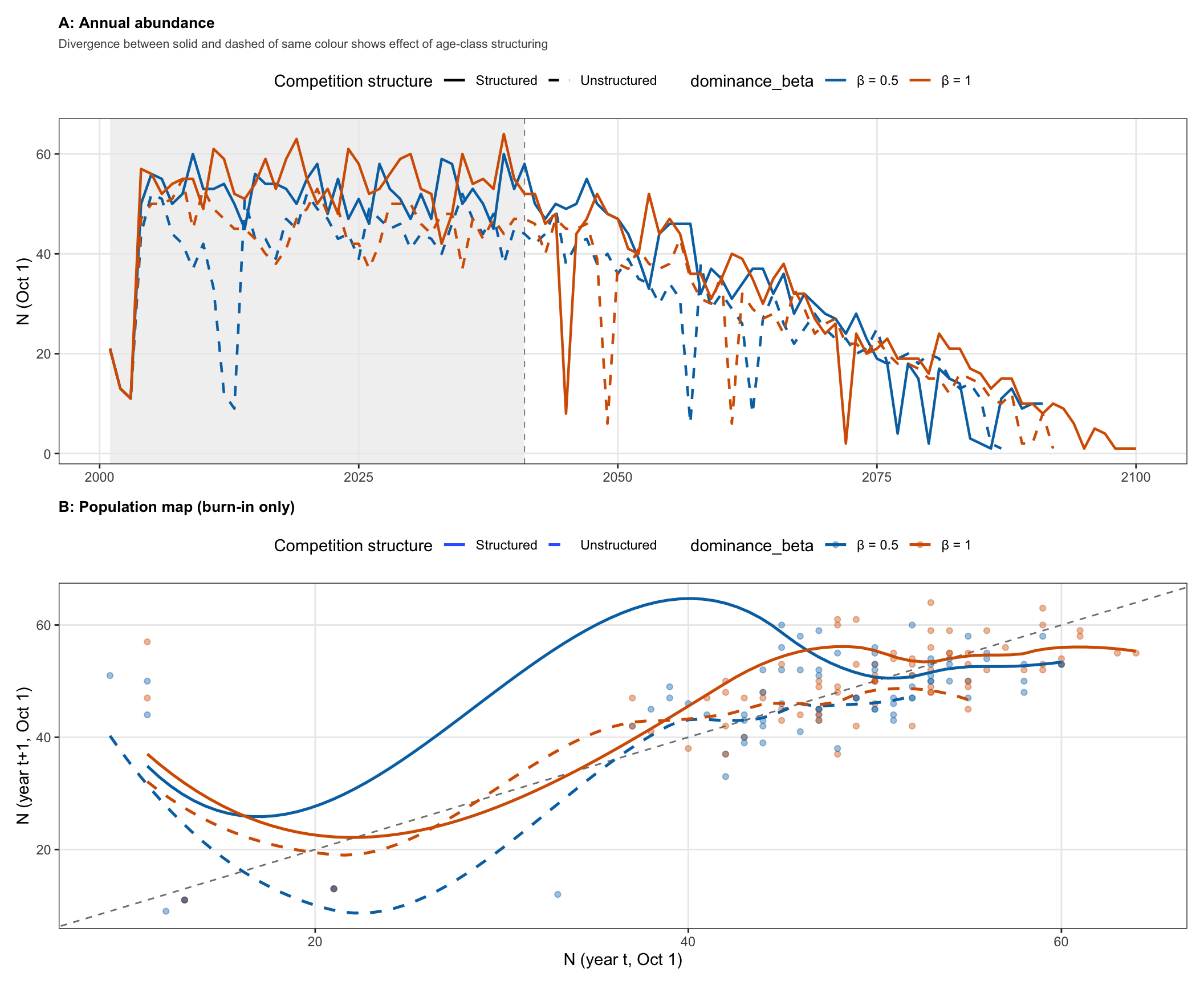
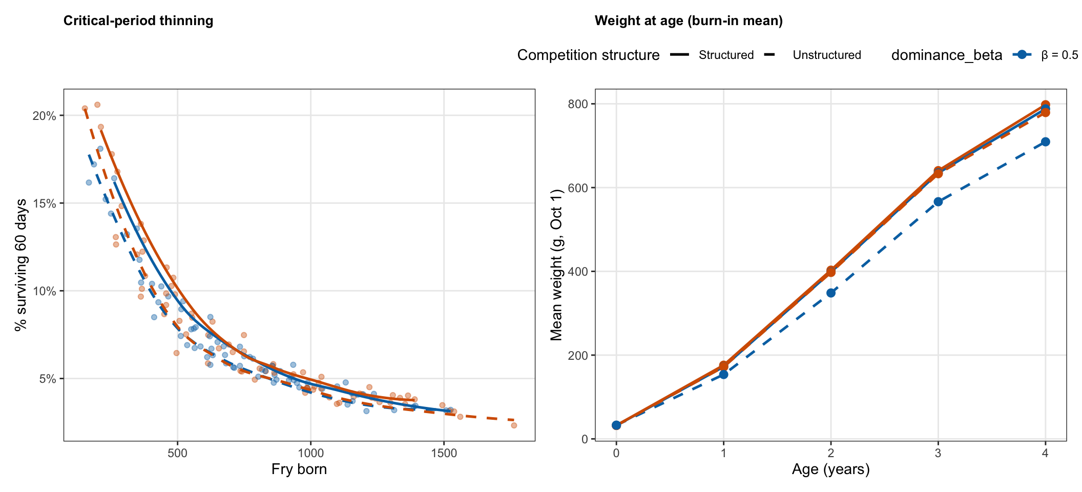
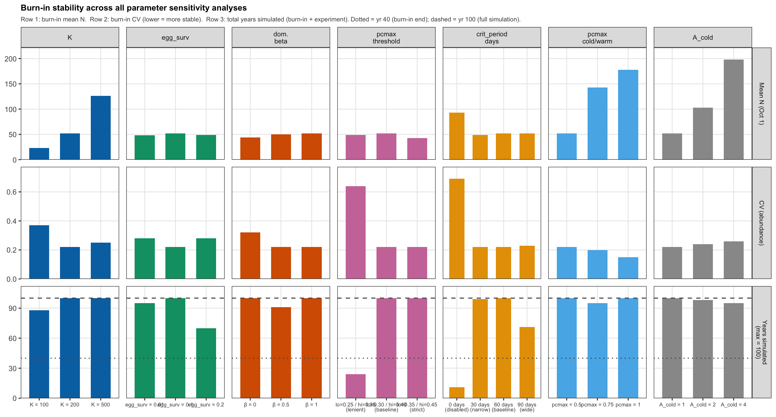
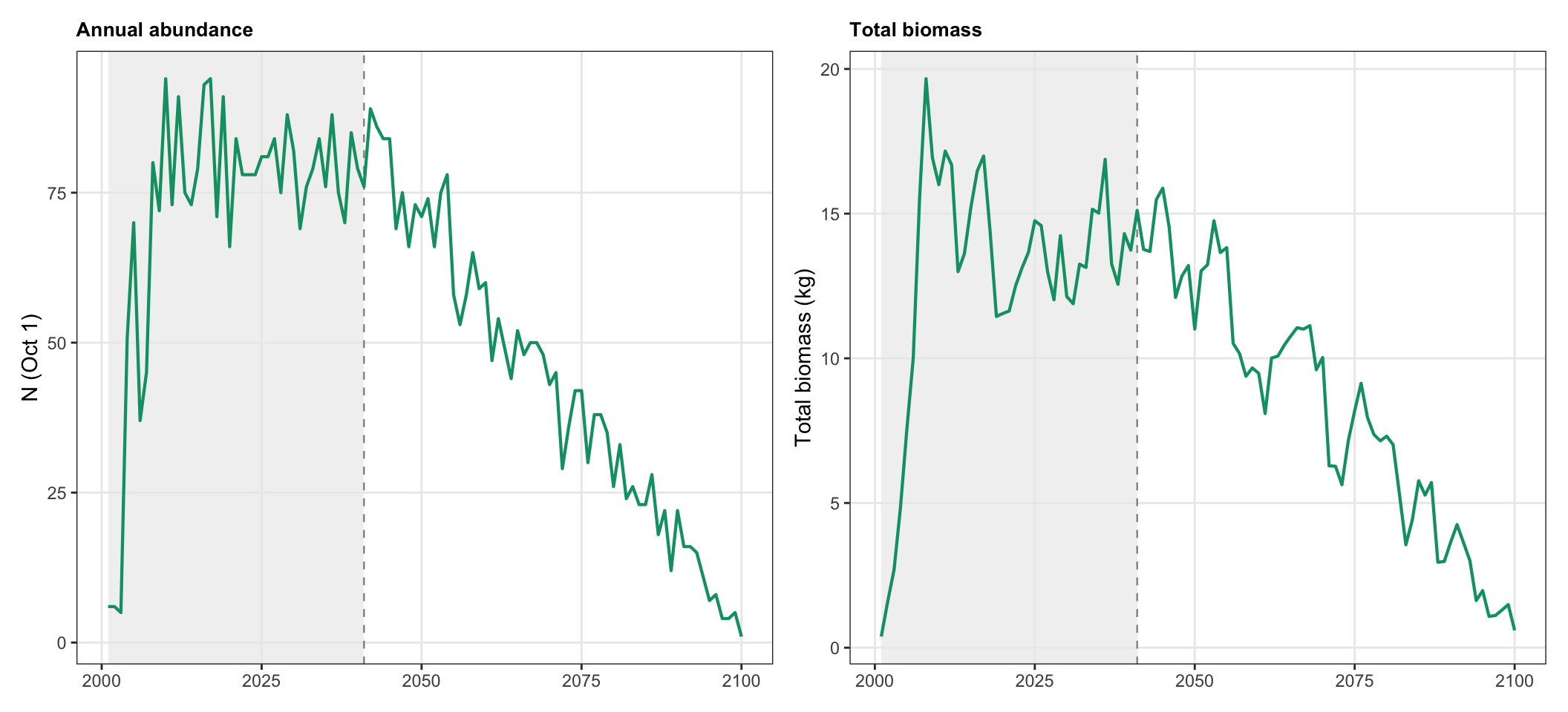
---
title: "Parameter Sensitivity Analysis"
subtitle: "Effects of key model parameters on population dynamics"
date: today
format:
html:
toc: true
toc-depth: 3
toc-title: "Contents"
code-fold: true
code-summary: "Show code"
theme: cosmo
fig-width: 11
fig-height: 7
execute:
warning: false
message: false
cache: true
---
```{r include=FALSE}
#| label: setup
#| cache: false
library(tidyverse)
library(lubridate)
library(patchwork)
source("Habitat.R")
source("Functions.R")
source("SimulationLoop.R")
source("ScenarioDefs.R")
```
```{r}
#| label: base parameters
#| cache: false
# ── Baseline parameter set ────────────────────────────────────────────────────
# All sensitivity runs keep every parameter at these values except the focal one.
baseline <- scenarios[["null_cold"]]

exp_start_date <- as.Date(baseline$mindate) + lubridate::years(baseline$nyears_burnin)
burn_start     <- year(as.Date(baseline$mindate))
exp_start_yr   <- year(exp_start_date)
exp_end_yr     <- exp_start_yr + baseline$nyears_experiment

cat("Baseline parameters:\n")
cat(" K_cold / K_warm :", baseline$K_cold, "/", baseline$K_warm, "\n")
cat(" egg_surv :", baseline$egg_surv, "\n")
cat(" dominance_beta :", baseline$dominance_beta, "\n")
cat(" pcmax_cold/warm :", baseline$pcmax_cold, "/", baseline$pcmax_warm, "\n")
cat(" A_cold/warm :", baseline$A_cold, "/", baseline$A_warm, "\n")
cat(" s_min :", baseline$s_min, "\n")
cat(" s_w0 :", baseline$s_w0, "\n")
cat(" s_k :", baseline$s_k, "\n")
cat(" age_structured_competition:", baseline$age_structured_competition, "\n")
cat("Burn-in:", burn_start, "–", exp_start_yr - 1,
    " | Experiment:", exp_start_yr, "–", exp_end_yr, "\n")
```
```{r}
#| label: helpers
#| cache: false
# ── Helper: run one sensitivity simulation ─────────────────────────────────────
run_sens <- function(param_name, param_val, base = baseline) {
  p   <- modifyList(base, setNames(list(param_val), param_name))
  # K must be set in both habitat and params
  if (param_name %in% c("K_cold", "K_warm")) {
    p <- modifyList(p, list(K_cold = param_val, K_warm = param_val))
  }
  hdf <- build_habitat(p)
  run_simulation(habitat_df = hdf, params = p, wt_growth = wt.growth)
}

# ── Helper: Oct 1 annual census (N and total biomass) ─────────────────────────
oct1_census <- function(sim, label) {
  sim$ibm_long |>
    filter(!is.na(date), survived == 1,
           month(date) == 10, day(date) == 1) |>
    mutate(year  = year(date),
           phase = if_else(year < exp_start_yr, "burn-in", "experiment")) |>
    group_by(year, phase) |>
    summarise(N        = n_distinct(pid),
              biomass_kg = sum(weight) / 1000,
              .groups  = "drop") |>
    mutate(label = label)
}

# ── Helper: population map (burn-in N[t+1] ~ N[t]) ───────────────────────────
pop_map <- function(census_df) {
  census_df |>
    filter(phase == "burn-in") |>
    group_by(label) |>
    arrange(year) |>
    mutate(N_next = lead(N)) |>
    ungroup() |>
    filter(!is.na(N_next))
}

# ── Helper: stock-recruitment (60-day survivor biomass vs spawner biomass) ─────
# Uses total biomass of fry on their 60th day of life as the recruitment metric.
# Biomass captures both the mortality effect (fewer survivors at high density)
# and the growth effect (survivors are lighter at high density due to food
# competition), giving a more complete picture of density-dependent compensation
# under the sigmoid fncSurviveSize than abundance alone would.
stock_recruit <- function(sim, label) {
  ibm <- sim$ibm_long
  hdf <- sim$habitat_df

  # Total biomass of fry on exactly their 60th day of life
  recruits_60d <- ibm |>
    filter(!is.na(parent_pid), !is.na(birth_dayofsim)) |>
    mutate(birth_yr    = year(hdf$date[birth_dayofsim]),
           day_of_life = dayofsim - birth_dayofsim) |>
    filter(birth_yr < exp_start_yr, day_of_life == 60) |>
    group_by(birth_yr) |>
    summarise(bio_surv60_kg = sum(weight) / 1000, .groups = "drop")

  # Spawner biomass: adults (≥ 100 g) present during spawning window (Apr–Jun)
  spawner_bio <- ibm |>
    filter(!is.na(date), survived == 1) |>
    mutate(year = year(date), doy = yday(date)) |>
    filter(doy >= 90, doy <= 150, weight >= 100, year < exp_start_yr) |>
    group_by(year) |>
    summarise(spawner_kg = sum(weight) / 1000, .groups = "drop")

  left_join(recruits_60d, spawner_bio, by = c("birth_yr" = "year")) |>
    mutate(label = label, spawner_kg = replace_na(spawner_kg, 0))
}

# ── Helper: size-based early thinning rate vs cohort size ─────────────────────
thinning_rate <- function(sim, label) {
  ibm <- sim$ibm_long
  hdf <- sim$habitat_df

  born <- ibm |>
    filter(!is.na(parent_pid)) |>
    mutate(birth_yr = year(hdf$date[birth_dayofsim])) |>
    filter(birth_yr < exp_start_yr) |>
    distinct(pid, birth_yr) |>
    count(birth_yr, name = "n_born")

  surv60 <- ibm |>
    filter(!is.na(parent_pid)) |>
    mutate(birth_yr = year(hdf$date[birth_dayofsim])) |>
    filter(birth_yr < exp_start_yr) |>
    group_by(pid, birth_yr) |>
    summarise(days_alive = n(), .groups = "drop") |>
    filter(days_alive >= 60) |>
    count(birth_yr, name = "n_surv60")

  left_join(born, surv60, by = "birth_yr") |>
    mutate(surv_rate = replace_na(n_surv60 / n_born, 0),
           label = label)
}

# ── Helper: biomass by age class (Oct 1, burn-in) ────────────────────────────
biomass_age <- function(sim, label) {
  sim$ibm_long |>
    filter(!is.na(date), survived == 1,
           month(date) == 10, day(date) == 1) |>
    mutate(year      = year(date),
           age_class = if_else(cohort == year, "Age-0 fry", "Age-1+"),
           phase     = if_else(year < exp_start_yr, "burn-in", "experiment")) |>
    filter(phase == "burn-in") |>
    group_by(year, age_class) |>
    summarise(biomass_kg = sum(weight) / 1000,
              n_fish     = n_distinct(pid), .groups = "drop") |>
    group_by(age_class) |>
    summarise(mean_bio_kg = mean(biomass_kg),
              mean_n      = mean(n_fish),
              mean_wt_g   = mean(biomass_kg * 1000 / pmax(n_fish, 1)),
              .groups = "drop") |>
    mutate(label = label)
}

# ── Helper: density–age-0 growth relationship (Aug 1 weight vs July density) ──
age0_density_growth <- function(sim, label) {
  ibm <- sim$ibm_long

  # Mean daily July abundance (all fish, all ages) per burn-in year
  july_dens <- ibm |>
    filter(!is.na(date), survived == 1, month(date) == 7,
           year(date) < exp_start_yr) |>
    group_by(year = year(date), date) |>
    summarise(n = n(), .groups = "drop") |>
    group_by(year) |>
    summarise(mean_july_n = mean(n), .groups = "drop")

  # Mean age-0 weight at Aug 1 (DOY 213) per burn-in cohort
  aug1_wt <- ibm |>
    filter(!is.na(date), survived == 1, !is.na(ggd),
           yday(date) == 213, year(date) < exp_start_yr) |>
    mutate(year = year(date)) |>
    filter(cohort == year) |>
    group_by(year) |>
    summarise(mean_wt = mean(weight), n = n(), .groups = "drop") |>
    filter(n >= 5)

  left_join(aug1_wt, july_dens, by = "year") |>
    mutate(label = label)
}

# ── Helper: weight-at-age (Oct 1, burn-in mean, ages 0-4) ────────────────────
wt_at_age <- function(sim, label) {
  sim$ibm_long |>
    filter(!is.na(date), survived == 1,
           month(date) == 10, day(date) == 1) |>
    mutate(year     = year(date),
           age_yrs  = floor(age),
           phase    = if_else(year < exp_start_yr, "burn-in", "experiment")) |>
    filter(phase == "burn-in", age_yrs <= 4) |>
    group_by(year, age_yrs) |>
    summarise(mean_wt = mean(weight), n = n_distinct(pid), .groups = "drop") |>
    filter(n >= 2) |>
    group_by(age_yrs) |>
    summarise(mean_wt = mean(mean_wt), .groups = "drop") |>
    mutate(label = label)
}

# ── Helper: age-0 daily weight (doy mean across burn-in cohorts) ──────────────
age0_daily_wt <- function(sim, label) {
  sim$ibm_long |>
    filter(!is.na(date), survived == 1, !is.na(ggd)) |>
    mutate(year = year(date),
           doy  = yday(date)) |>
    filter(cohort == year, year < exp_start_yr) |>
    group_by(doy) |>
    summarise(mean_wt = mean(weight), n = n(), .groups = "drop") |>
    filter(n >= 5) |>
    mutate(label = label)
}

# ── Stability summary ──────────────────────────────────────────────────────────
stability_stats <- function(census_df) {
  census_df |>
    group_by(label, phase) |>
    summarise(mean_N     = round(mean(N)),
              cv         = round(sd(N) / mean(N), 2),
              mean_bio   = round(mean(biomass_kg), 1),
              sim_yrs    = n(),
              .groups    = "drop")
}

# ── Total years simulated (burn-in + experiment combined) ─────────────────────
# Used in the cross-parameter summary to identify premature collapse.
# max possible = nyears_burnin + nyears_experiment = 100.
total_sim_yrs <- function(census_df) {
  census_df |>
    group_by(label) |>
    summarise(total_yrs = n_distinct(year), .groups = "drop")
}

# ── Helper: 4-panel stability bar chart (mean N and CV × phase) ───────────────
# stable_df: output of stability_stats(); cols: length-3 colour vector.
# Layout: rows = metric (mean N, CV), columns = phase (burn-in, experiment).
plot_stability_fig <- function(stable_df, cols) {
  stable_long <- stable_df |>
    select(label, phase, mean_N, cv) |>
    pivot_longer(c(mean_N, cv),
                 names_to  = "metric",
                 values_to = "value") |>
    mutate(
      metric = factor(metric,
                      levels = c("mean_N", "cv"),
                      labels = c("Mean N (Oct 1)", "CV (abundance)")),
      phase  = factor(phase,
                      levels = c("burn-in", "experiment"),
                      labels = c("Burn-in", "Experiment"))
    )

  ggplot(stable_long, aes(x = label, y = value, fill = label)) +
    geom_col(width = 0.65, show.legend = FALSE) +
    facet_grid(metric ~ phase, scales = "free_y") +
    scale_fill_manual(values = cols) +
    labs(x = NULL, y = NULL) +
    theme_sens() +
    theme(axis.text.x  = element_text(size = 7.5, lineheight = 0.85),
          strip.text   = element_text(size = 9),
          panel.spacing = unit(0.8, "lines"))
}

# ── Helper: days post-hatch until cohort-mean weight first exceeds s_w0 ───────
# Reads s_w0 from sim$params so it works for any parameter section:
# — non-s_w0 sections: all sims share the baseline s_w0 (one threshold line)
# — s_w0 section: each sim has its own s_w0 (three threshold lines)
days_to_threshold <- function(sim, label) {
  ibm    <- sim$ibm_long
  hdf    <- sim$habitat_df
  w0_val <- sim$params$s_w0

  cohort_wt <- ibm |>
    filter(!is.na(date), survived == 1, !is.na(ggd),
           year(date) < exp_start_yr) |>
    mutate(doy = yday(date)) |>
    filter(cohort == year(date)) |>
    group_by(cohort, doy) |>
    summarise(mean_wt = mean(weight), n = n(), .groups = "drop") |>
    filter(n >= 5)

  threshold_doy <- cohort_wt |>
    group_by(cohort) |>
    summarise(
      hatch_doy   = min(doy),
      cross_doy   = doy[which(mean_wt >= w0_val)[1]],
      .groups     = "drop"
    ) |>
    mutate(days_to_cross = cross_doy - hatch_doy)

  fry_born <- sim$spawn_log |>
    left_join(hdf |> select(dayofsim, date), by = "dayofsim") |>
    filter(!is.na(date), year(date) < exp_start_yr) |>
    mutate(cohort = year(date)) |>
    group_by(cohort) |>
    summarise(n_born = sum(n_offspring), .groups = "drop")

  left_join(threshold_doy, fry_born, by = "cohort") |>
    filter(!is.na(days_to_cross), !is.na(n_born)) |>
    mutate(label = label, w0 = w0_val)
}

# ── Helper: scatter + OLS plot of days-to-threshold vs fry born ───────────────
plot_danger_duration <- function(cross_df, cols) {
  slope_labs <- cross_df |>
    group_by(label, w0) |>
    summarise(
      slope = coef(lm(days_to_cross ~ n_born))[["n_born"]] * 1000,
      r_sq  = summary(lm(days_to_cross ~ n_born))$r.squared,
      .groups = "drop"
    ) |>
    arrange(w0) |>
    mutate(
      x   = max(cross_df$n_born, na.rm = TRUE) * 0.97,
      y   = seq(
        from       = quantile(cross_df$days_to_cross, 0.38, na.rm = TRUE),
        by         = diff(range(cross_df$days_to_cross, na.rm = TRUE)) * 0.15,
        length.out = n()
      ),
      txt = paste0("+", round(slope, 1), " d / 1000 fry  (R\u00b2 = ", round(r_sq, 2), ")")
    )

  ggplot(cross_df, aes(x = n_born, y = days_to_cross, color = label)) +
    geom_point(alpha = 0.55, size = 2) +
    geom_smooth(method = "lm", se = TRUE, linewidth = 0.9, alpha = 0.12) +
    # geom_text(data = slope_labs,
    #           aes(x = x, y = y, label = txt, color = label),
    #           hjust = 1, size = 2.8, fontface = "italic", show.legend = FALSE) +
    scale_color_manual(values = cols) +
    scale_x_continuous(labels = scales::comma) +
    labs(x     = "Fry born (cohort size)",
         y     = "Days post-hatch to exceed s_w0",
         color = NULL,
         title = "Density extends the low-survival window") +
    theme_sens()
}

# ── Shared colour palette (Okabe-Ito: blue / teal / vermillion) ──────────────
# Colorblind-friendly; all three are clearly distinguishable.
# Mapping: low value = blue, mid/baseline value = teal, high value = vermillion.
sens_cols <- c("#0072B2", "#009E73", "#D55E00")

# ── Shared plot theme ─────────────────────────────────────────────────────────
theme_sens <- function() {
  theme_bw() +
    theme(legend.position  = "top",
          strip.background = element_rect(fill = "grey88"),
          panel.grid.minor = element_blank(),
          plot.title       = element_text(size = 10, face = "bold"),
          plot.subtitle    = element_text(size = 8, color = "grey30"))
}
```
---
## `K_cold`: strength of density dependence
The half-saturation constant K controls the density at which consumption suppression
becomes binding. Smaller K creates stronger suppression at lower densities; larger K
allows the population to grow more before density effects manifest.
```{r}
#| label: sim-K
#| cache: true
K_vals   <- c(100, 200, 500)
K_labels <- paste0("K = ", K_vals)
K_cols   <- sens_cols

cat("Running K sensitivity simulations...\n")
K_sims <- lapply(seq_along(K_vals), function(i) {
  cat(" K =", K_vals[i], "... ")
  p   <- modifyList(baseline, list(K_cold = K_vals[i], K_warm = K_vals[i]))
  hdf <- build_habitat(p)
  res <- run_simulation(hdf, p, wt_growth = wt.growth)
  cat("ends", format(max(res$ibm_long$date, na.rm = TRUE)), "\n")
  res
})
names(K_sims) <- K_labels
```
```{r}
#| label: K-outcomes
K_census   <- bind_rows(Map(oct1_census,   K_sims, K_labels)) |>
  mutate(label = factor(label, levels = K_labels))
K_sr       <- bind_rows(Map(stock_recruit, K_sims, K_labels)) |>
  mutate(label = factor(label, levels = K_labels))
K_thin     <- bind_rows(Map(thinning_rate,        K_sims, K_labels)) |>
  mutate(label = factor(label, levels = K_labels))
K_dg       <- bind_rows(Map(age0_density_growth, K_sims, K_labels)) |>
  mutate(label = factor(label, levels = K_labels))

K_waa      <- bind_rows(Map(wt_at_age,     K_sims, K_labels)) |>
  mutate(label = factor(label, levels = K_labels))
K_age0_dly <- bind_rows(Map(age0_daily_wt, K_sims, K_labels)) |>
  mutate(label = factor(label, levels = K_labels))
K_stable   <- stability_stats(K_census)
```
### Abundance and biomass
```{r}
#| label: fig-K-ts
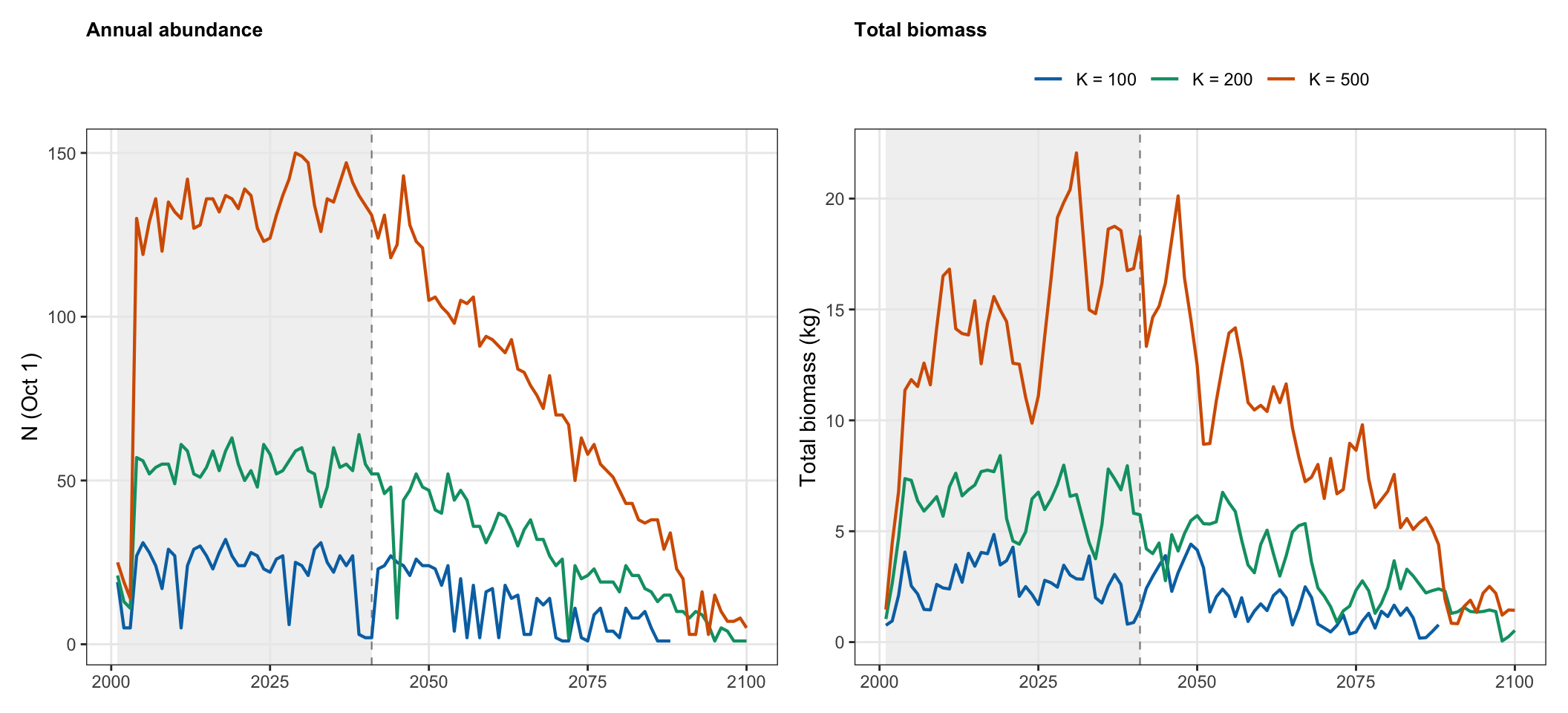
#| fig-cap: "Oct 1 annual abundance and total biomass for each K value. Grey band = burn-in."
#| fig-height: 5
p_N <- ggplot(K_census, aes(x = year, y = N, color = label)) +
  annotate("rect", xmin = burn_start, xmax = exp_start_yr,
           ymin = -Inf, ymax = Inf, fill = "grey92", alpha = 0.7) +
  geom_vline(xintercept = exp_start_yr, linetype = "dashed",
             color = "grey55", linewidth = 0.4) +
  geom_line(linewidth = 0.75) +
  scale_color_manual(values = K_cols) +
  labs(x = NULL, y = "N (Oct 1)", color = NULL, title = "Annual abundance") +
  theme_sens() + theme(legend.position = "none")

p_B <- ggplot(K_census, aes(x = year, y = biomass_kg, color = label)) +
  annotate("rect", xmin = burn_start, xmax = exp_start_yr,
           ymin = -Inf, ymax = Inf, fill = "grey92", alpha = 0.7) +
  geom_vline(xintercept = exp_start_yr, linetype = "dashed",
             color = "grey55", linewidth = 0.4) +
  geom_line(linewidth = 0.75) +
  scale_color_manual(values = K_cols) +
  labs(x = NULL, y = "Total biomass (kg)", color = NULL, title = "Total biomass") +
  theme_sens()

p_N | p_B
```
### Compensatory dynamics
```{r}
#| label: fig-K-comp
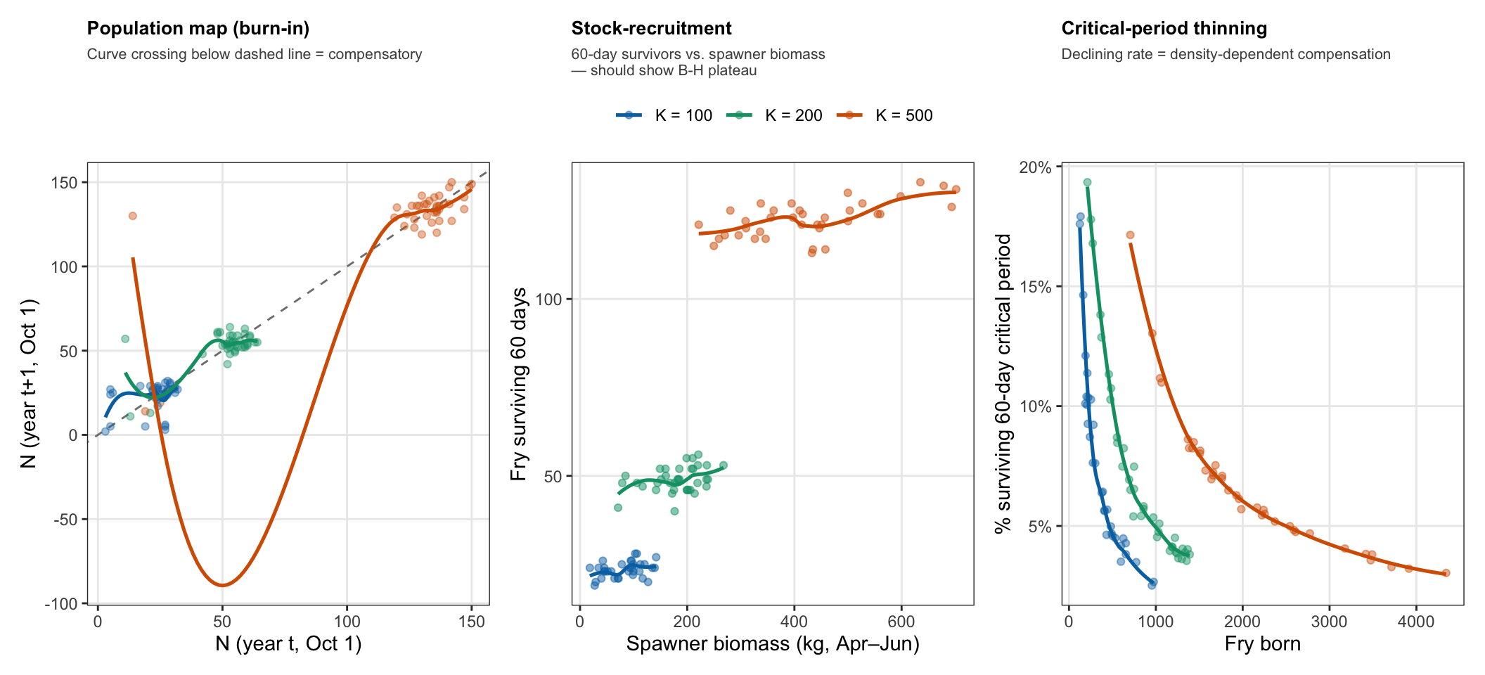
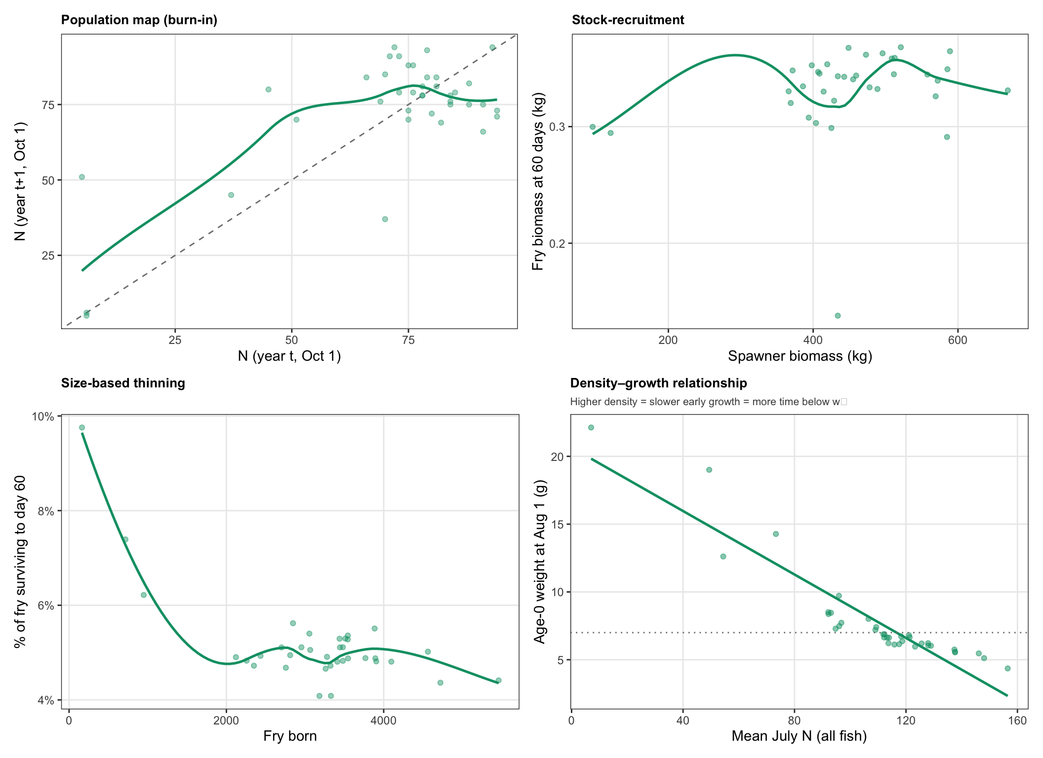
#| fig-cap: "Top-left: burn-in population map. Top-right: stock-recruitment relationship. Bottom-left: size-based early thinning (% of fry surviving to day 60). Bottom-right: density–growth relationship (age-0 weight at Aug 1 vs July abundance). The bottom row together shows the two pathways of size-based density-dependent compensation: cohort thinning (left) and growth suppression (right)."
#| fig-height: 8
K_map <- pop_map(K_census)

p_map <- ggplot(K_map, aes(x = N, y = N_next, color = label)) +
  geom_abline(slope = 1, intercept = 0, linetype = "dashed", color = "grey50") +
  geom_point(alpha = 0.4, size = 1.5) +
  geom_smooth(method = "loess", se = FALSE, span = 0.75, linewidth = 0.9) +
  scale_color_manual(values = K_cols) +
  labs(x = "N (year t, Oct 1)", y = "N (year t+1, Oct 1)", color = NULL,
       title = "Population map (burn-in)",
       subtitle = "Curve crossing below dashed line = compensatory") +
  theme_sens() + theme(legend.position = "none")

p_sr <- ggplot(K_sr |> filter(spawner_kg > 0),
               aes(x = spawner_kg, y = bio_surv60_kg, color = label)) +
  geom_point(alpha = 0.5, size = 1.5) +
  geom_smooth(method = "loess", se = FALSE, span = 0.7, linewidth = 0.9) +
  scale_color_manual(values = K_cols) +
  labs(x = "Spawner biomass (kg, Apr–Jun)", y = "Fry biomass at 60 days (kg)",
       color = NULL, title = "Stock-recruitment",
       subtitle = "60-day survivor biomass vs. spawner biomass \n— should show B-H plateau") +
  theme_sens() + theme(legend.position = "right")

p_thin <- ggplot(K_thin, aes(x = n_born, y = surv_rate, color = label)) +
  geom_point(alpha = 0.45, size = 1.5) +
  geom_smooth(method = "loess", se = FALSE, span = 0.7, linewidth = 0.9) +
  scale_y_continuous(labels = scales::percent_format(accuracy = 1)) +
  scale_color_manual(values = K_cols) +
  labs(x = "Fry born", y = "% of fry surviving to day 60",
       color = NULL, title = "Size-based thinning",
       subtitle = "Declining rate = density-dependent compensation") +
  theme_sens() + theme(legend.position = "none")

p_dg <- ggplot(K_dg, aes(x = mean_july_n, y = mean_wt, color = label)) +
  geom_point(alpha = 0.5, size = 1.5) +
  geom_smooth(method = "lm", se = FALSE, linewidth = 0.9) +
  geom_hline(yintercept = 7, linetype = "dotted", color = "grey50") +
  scale_color_manual(values = K_cols) +
  labs(x = "Mean July N (all fish)", y = "Age-0 weight at Aug 1 (g)", color = NULL,
       title = "Density\u2013growth relationship",
       subtitle = "Higher density = slower early growth = more time below w\u2080") +
  theme_sens() + theme(legend.position = "none")

(p_map | p_sr) / (p_thin | p_dg)
```
### Age structure
```{r}
#| label: fig-K-thin
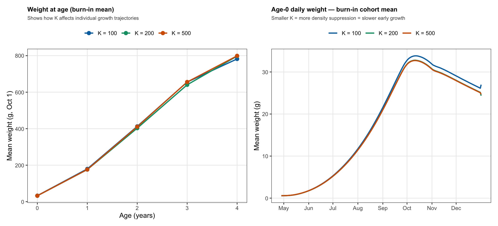
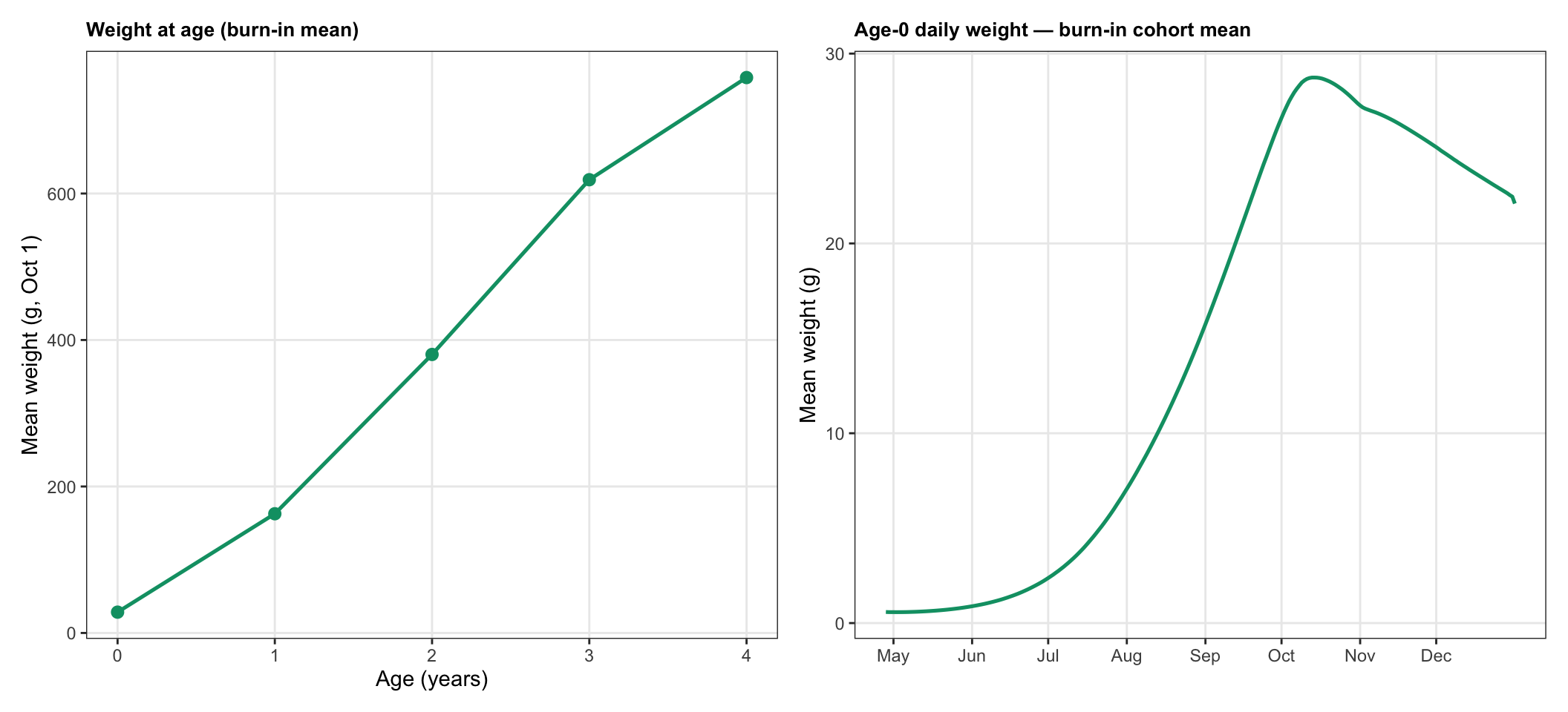
#| fig-cap: "Left: mean weight at age (burn-in). Right: Mean age-0 fry weight by day of year, averaged across burn-in cohorts."
#| fig-height: 5
p_waa <- ggplot(K_waa, aes(x = age_yrs, y = mean_wt, color = label)) +
  geom_line(linewidth = 0.9) +
  geom_point(size = 2.5) +
  scale_color_manual(values = K_cols) +
  scale_x_continuous(breaks = 0:4) +
  labs(x = "Age (years)", y = "Mean weight (g, Oct 1)",
       color = NULL, title = "Weight at age (burn-in mean)",
       subtitle = "Shows how K affects individual growth trajectories") +
  theme_sens()

month_doys   <- c(121, 152, 182, 213, 244, 274, 305, 335)
month_labels <- c("May","Jun","Jul","Aug","Sep","Oct","Nov","Dec")

p_aget <- ggplot(K_age0_dly |> filter(doy >= 118),
       aes(x = doy, y = mean_wt, color = label)) +
  geom_line(linewidth = 0.9) +
  scale_color_manual(values = K_cols) +
  scale_x_continuous(breaks = month_doys, labels = month_labels) +
  labs(x = NULL, y = "Mean weight (g)", color = NULL,
       title = "Age-0 daily weight — burn-in cohort mean",
       subtitle = "Smaller K = more density suppression = slower early growth") +
  theme_sens()

p_waa | p_aget
```
### Density-dependent duration below s_w0
```{r}
#| label: fig-K-danger-duration
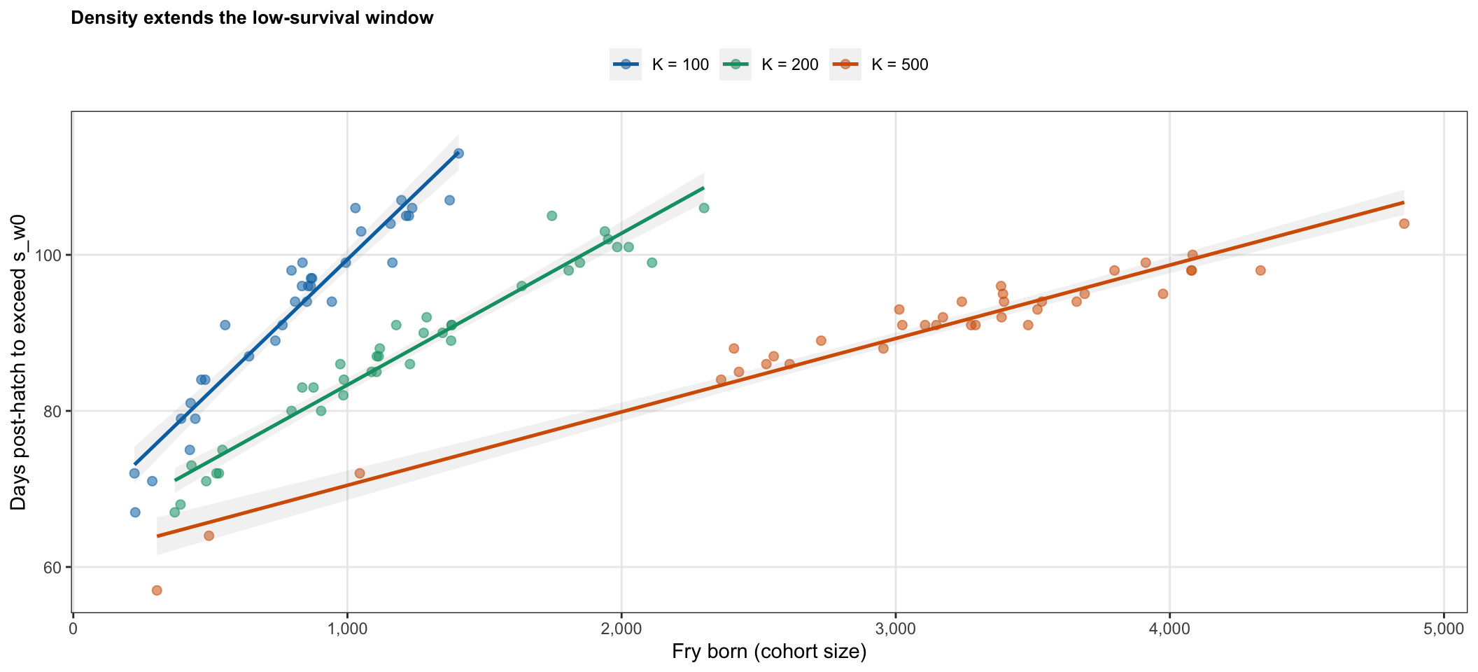
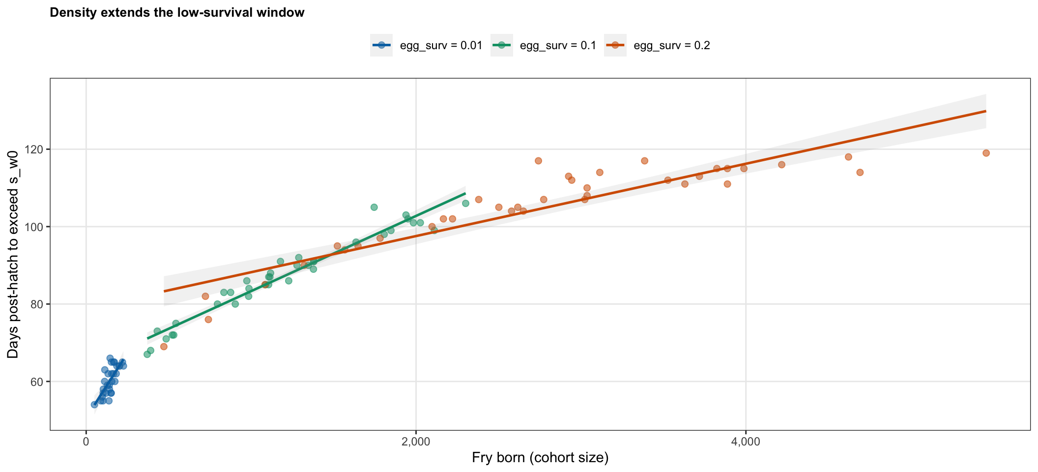
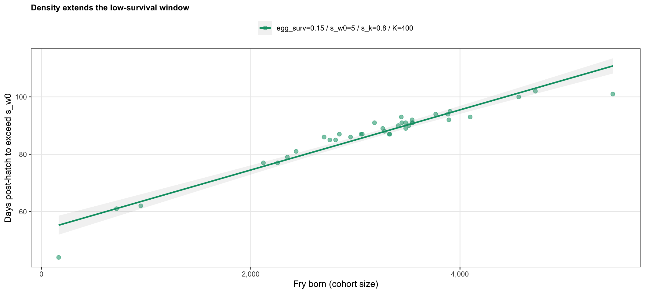
#| fig-cap: "Days post-hatch until cohort-mean weight first exceeds s_w0, vs fry born. Each point is one burn-in cohort year; lines are OLS fits with 95% CI."
#| fig-height: 5
K_cross <- bind_rows(Map(days_to_threshold, K_sims, K_labels)) |>
  mutate(label = factor(label, levels = K_labels))

plot_danger_duration(K_cross, K_cols)
```
### Stability summary {.unnumbered}
```{r}
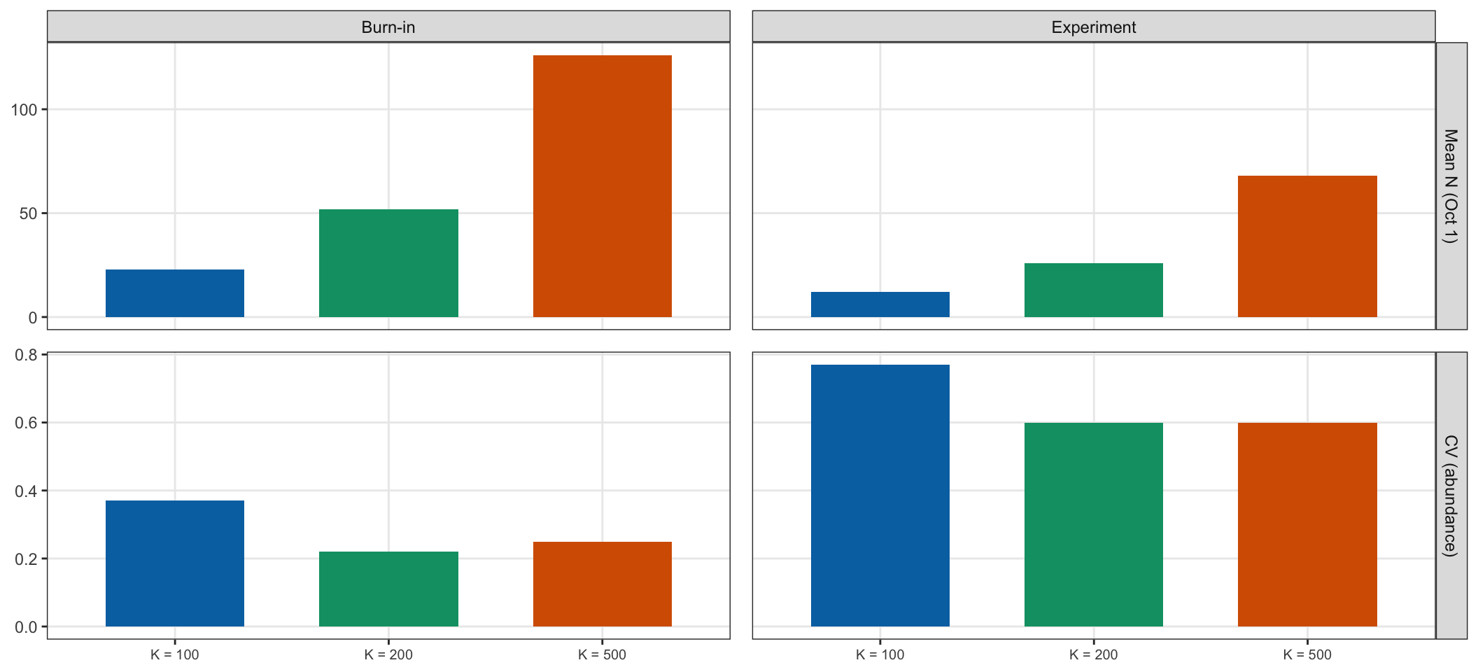
#| label: fig-K-stable
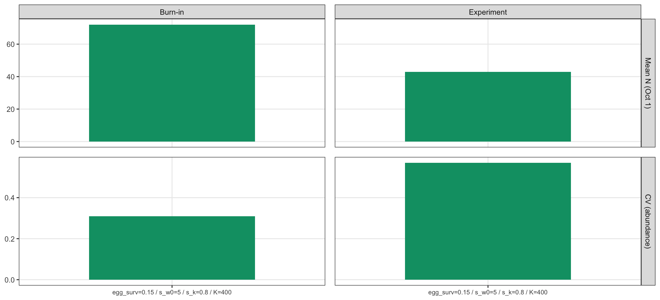
#| fig-cap: "Mean Oct 1 abundance and CV by K value, split by simulation phase."
#| fig-height: 5
plot_stability_fig(K_stable, K_cols)
```
```{r}
#| label: tbl-K-stable
#| tbl-cap: "Burn-in and experiment stability statistics by K value."
K_stable |>
  knitr::kable(col.names = c("K", "Phase", "Mean N",
                              "CV (abundance)", "Mean biomass (kg)", "Years"))
```
---
## `egg_surv`: proportional egg survival
Egg-to-fry survival scales the number of recruits entering the simulation each spring.
It represents spawning habitat quality, redd conditions, and egg-incubation success.
```{r}
#| label: sim-egg
#| cache: true
egg_vals   <- c(0.01, 0.1, 0.2)
egg_labels <- paste0("egg_surv = ", egg_vals)
egg_cols   <- sens_cols

cat("Running egg_surv sensitivity simulations...\n")
egg_sims <- lapply(seq_along(egg_vals), function(i) {
  cat(" egg_surv =", egg_vals[i], "... ")
  p   <- modifyList(baseline, list(egg_surv = egg_vals[i]))
  hdf <- build_habitat(p)
  res <- run_simulation(hdf, p, wt_growth = wt.growth)
  cat("ends", format(max(res$ibm_long$date, na.rm = TRUE)), "\n")
  res
})
names(egg_sims) <- egg_labels
```
```{r}
#| label: egg-outcomes
egg_census   <- bind_rows(Map(oct1_census,   egg_sims, egg_labels)) |>
  mutate(label = factor(label, levels = egg_labels))
egg_sr       <- bind_rows(Map(stock_recruit, egg_sims, egg_labels)) |>
  mutate(label = factor(label, levels = egg_labels))
egg_thin     <- bind_rows(Map(thinning_rate,        egg_sims, egg_labels)) |>
  mutate(label = factor(label, levels = egg_labels))
egg_dg       <- bind_rows(Map(age0_density_growth, egg_sims, egg_labels)) |>
  mutate(label = factor(label, levels = egg_labels))

egg_waa      <- bind_rows(Map(wt_at_age,     egg_sims, egg_labels)) |>
  mutate(label = factor(label, levels = egg_labels))
egg_age0_dly <- bind_rows(Map(age0_daily_wt, egg_sims, egg_labels)) |>
  mutate(label = factor(label, levels = egg_labels))
egg_stable   <- stability_stats(egg_census)
```
### Abundance and biomass
```{r}
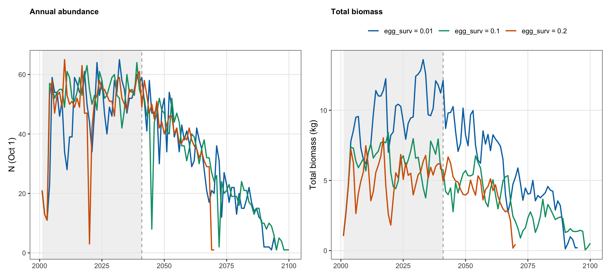
#| label: fig-egg-ts
#| fig-cap: "Oct 1 annual abundance and total biomass for each egg_surv value."
#| fig-height: 5
p_N <- ggplot(egg_census, aes(x = year, y = N, color = label)) +
  annotate("rect", xmin = burn_start, xmax = exp_start_yr,
           ymin = -Inf, ymax = Inf, fill = "grey92", alpha = 0.7) +
  geom_vline(xintercept = exp_start_yr, linetype = "dashed",
             color = "grey55", linewidth = 0.4) +
  geom_line(linewidth = 0.75) +
  scale_color_manual(values = egg_cols) +
  labs(x = NULL, y = "N (Oct 1)", color = NULL, title = "Annual abundance") +
  theme_sens() + theme(legend.position = "none")

p_B <- ggplot(egg_census, aes(x = year, y = biomass_kg, color = label)) +
  annotate("rect", xmin = burn_start, xmax = exp_start_yr,
           ymin = -Inf, ymax = Inf, fill = "grey92", alpha = 0.7) +
  geom_vline(xintercept = exp_start_yr, linetype = "dashed",
             color = "grey55", linewidth = 0.4) +
  geom_line(linewidth = 0.75) +
  scale_color_manual(values = egg_cols) +
  labs(x = NULL, y = "Total biomass (kg)", color = NULL, title = "Total biomass") +
  theme_sens()

p_N | p_B
```
### Compensatory dynamics
```{r}
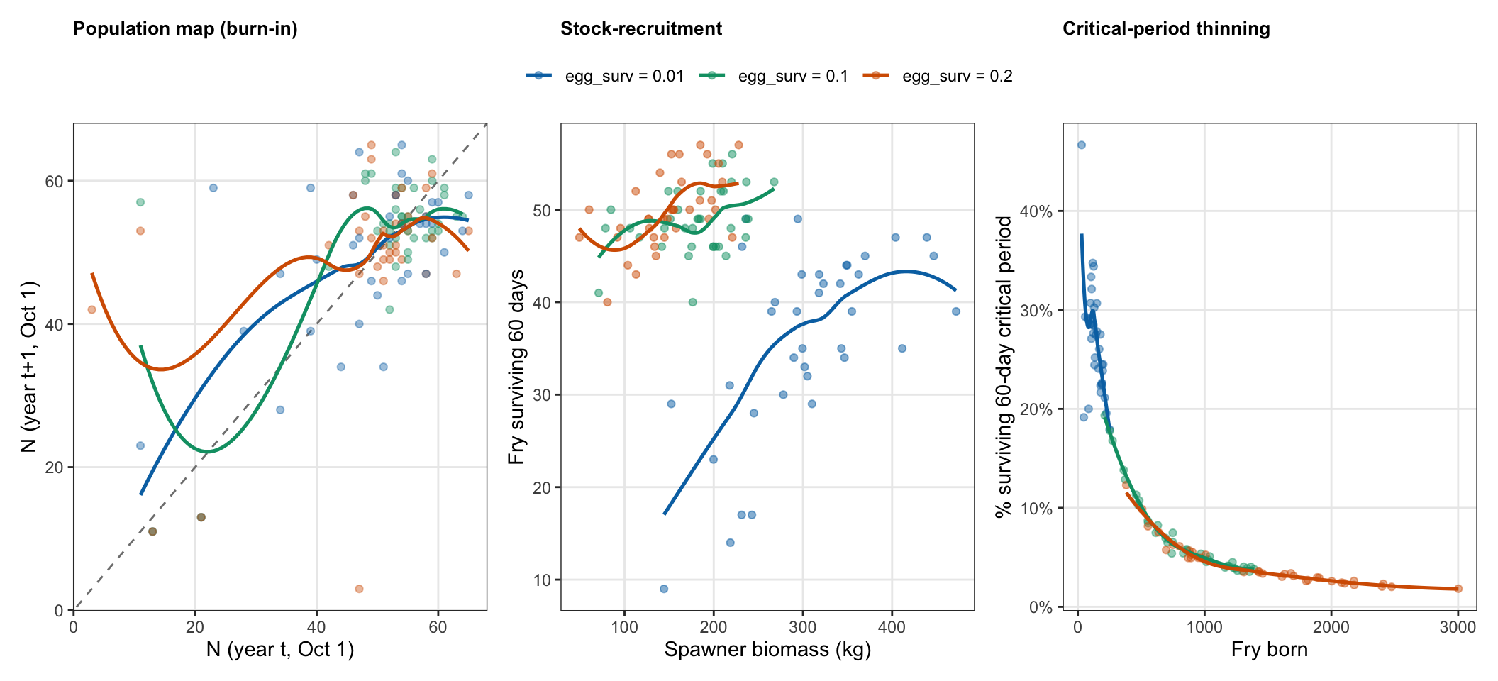
#| label: fig-egg-comp
#| fig-cap: "Top-left: burn-in population map. Top-right: stock-recruitment. Bottom-left: size-based early thinning (% of fry surviving to day 60). Bottom-right: density–growth relationship. The bottom row together shows the two pathways of size-based density-dependent compensation: cohort thinning (left) and growth suppression (right)."
#| fig-height: 8
egg_map <- pop_map(egg_census)

p_map <- ggplot(egg_map, aes(x = N, y = N_next, color = label)) +
  geom_abline(slope = 1, intercept = 0, linetype = "dashed", color = "grey50") +
  geom_point(alpha = 0.4, size = 1.5) +
  geom_smooth(method = "loess", se = FALSE, span = 0.75, linewidth = 0.9) +
  scale_color_manual(values = egg_cols) +
  labs(x = "N (year t, Oct 1)", y = "N (year t+1, Oct 1)", color = NULL,
       title = "Population map (burn-in)") +
  theme_sens() + theme(legend.position = "none")

p_sr <- ggplot(egg_sr |> filter(spawner_kg > 0),
               aes(x = spawner_kg, y = bio_surv60_kg, color = label)) +
  geom_point(alpha = 0.5, size = 1.5) +
  geom_smooth(method = "loess", se = FALSE, span = 0.7, linewidth = 0.9) +
  scale_color_manual(values = egg_cols) +
  labs(x = "Spawner biomass (kg)", y = "Fry biomass at 60 days (kg)",
       color = NULL, title = "Stock-recruitment") +
  theme_sens() + theme(legend.position = "right")

p_thin <- ggplot(egg_thin, aes(x = n_born, y = surv_rate, color = label)) +
  geom_point(alpha = 0.45, size = 1.5) +
  geom_smooth(method = "loess", se = FALSE, span = 0.7, linewidth = 0.9) +
  scale_y_continuous(labels = scales::percent_format(accuracy = 1)) +
  scale_color_manual(values = egg_cols) +
  labs(x = "Fry born", y = "% of fry surviving to day 60",
       color = NULL, title = "Size-based thinning") +
  theme_sens() + theme(legend.position = "none")

p_dg <- ggplot(egg_dg, aes(x = mean_july_n, y = mean_wt, color = label)) +
  geom_point(alpha = 0.5, size = 1.5) +
  geom_smooth(method = "lm", se = FALSE, linewidth = 0.9) +
  geom_hline(yintercept = 7, linetype = "dotted", color = "grey50") +
  scale_color_manual(values = egg_cols) +
  labs(x = "Mean July N (all fish)", y = "Age-0 weight at Aug 1 (g)", color = NULL,
       title = "Density\u2013growth relationship",
       subtitle = "Higher density = slower early growth = more time below w\u2080") +
  theme_sens() + theme(legend.position = "none")

(p_map | p_sr) / (p_thin | p_dg)
```
### Age structure
```{r}
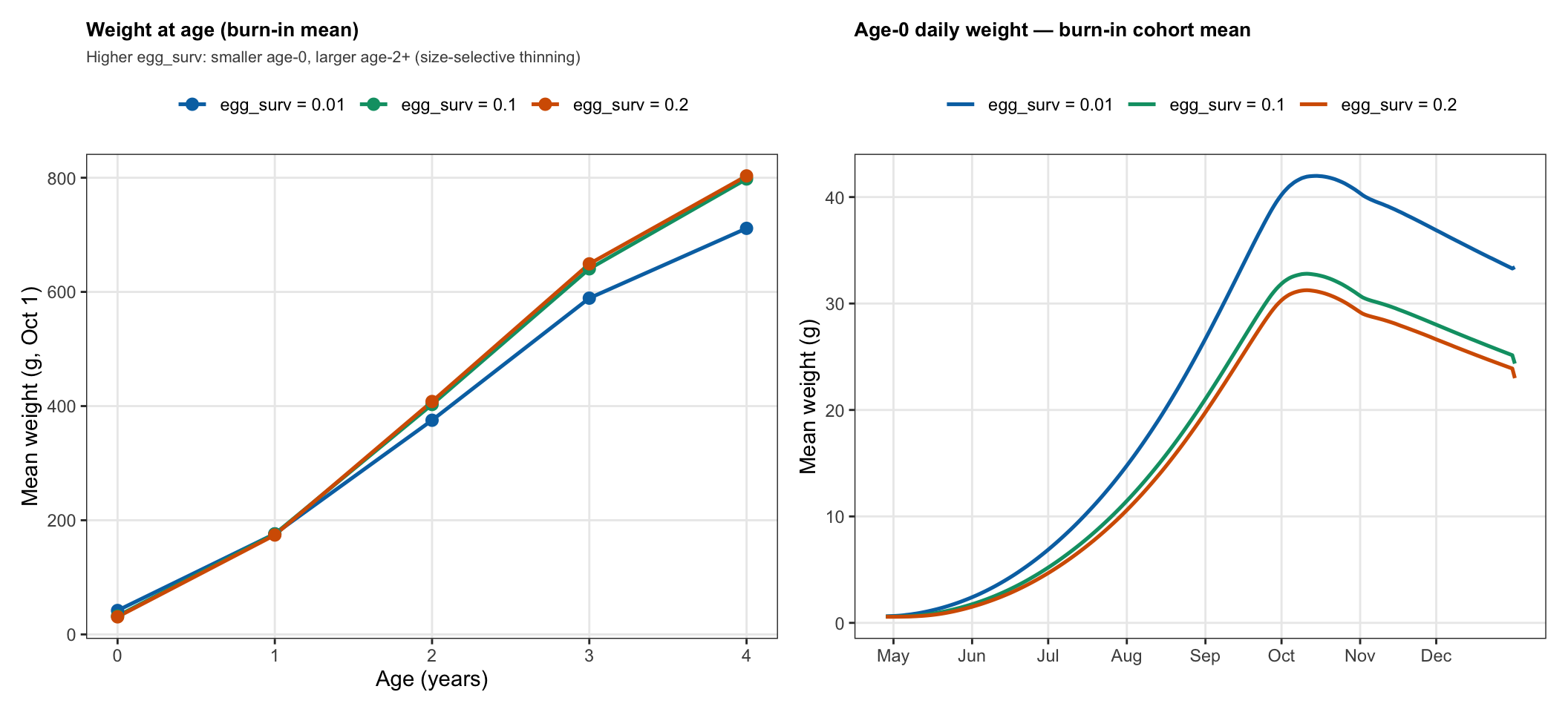
#| label: fig-egg-age0
#| fig-cap: "Left: mean weight at age (burn-in). Right: age-0 daily weight by day of year, averaged across burn-in cohorts."
#| fig-height: 5
p_waa <- ggplot(egg_waa, aes(x = age_yrs, y = mean_wt, color = label)) +
  geom_line(linewidth = 0.9) +
  geom_point(size = 2.5) +
  scale_color_manual(values = egg_cols) +
  scale_x_continuous(breaks = 0:4) +
  labs(x = "Age (years)", y = "Mean weight (g, Oct 1)",
       color = NULL, title = "Weight at age (burn-in mean)",
       subtitle = "Higher egg_surv: smaller age-0, larger age-2+ (size-selective thinning)") +
  theme_sens()

p_aget <- ggplot(egg_age0_dly |> filter(doy >= 118),
                 aes(x = doy, y = mean_wt, color = label)) +
  geom_line(linewidth = 0.9) +
  scale_color_manual(values = egg_cols) +
  scale_x_continuous(breaks = month_doys, labels = month_labels) +
  labs(x = NULL, y = "Mean weight (g)", color = NULL,
       title = "Age-0 daily weight — burn-in cohort mean") +
  theme_sens()

p_waa | p_aget
```
### Density-dependent duration below s_w0
```{r}
#| label: fig-egg-danger-duration
#| fig-cap: "Days post-hatch until cohort-mean weight first exceeds s_w0, vs fry born. Each point is one burn-in cohort year; lines are OLS fits with 95% CI."
#| fig-height: 5
egg_cross <- bind_rows(Map(days_to_threshold, egg_sims, egg_labels)) |>
  mutate(label = factor(label, levels = egg_labels))

plot_danger_duration(egg_cross, egg_cols)
```
### Stability summary {.unnumbered}
```{r}
#| label: fig-egg-stable
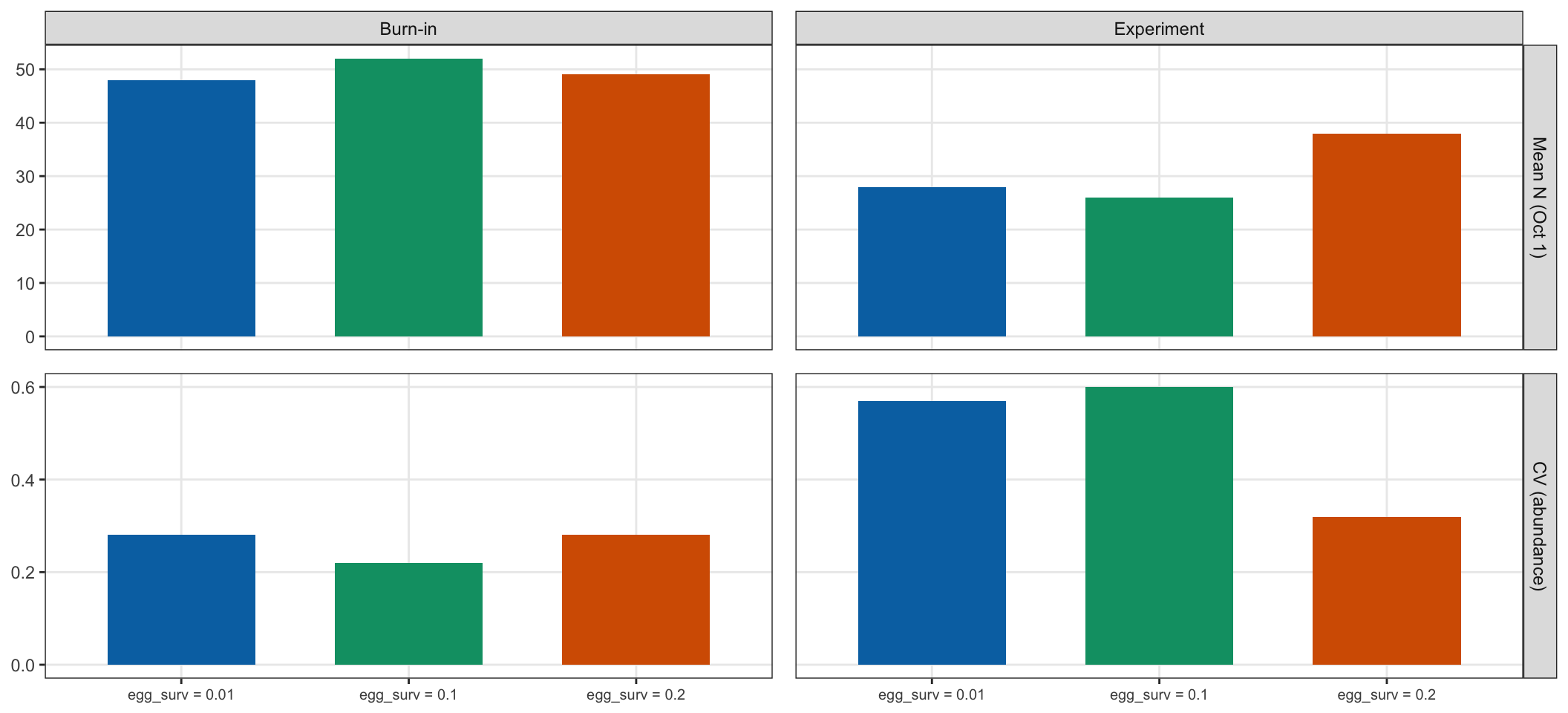
#| fig-cap: "Mean Oct 1 abundance and CV by egg_surv, split by simulation phase."
#| fig-height: 5
plot_stability_fig(egg_stable, egg_cols)
```
```{r}
#| label: tbl-egg-stable
#| tbl-cap: "Stability statistics by egg_surv."
egg_stable |>
  knitr::kable(col.names = c("egg_surv", "Phase", "Mean N",
                              "CV (abundance)", "Mean biomass (kg)", "Years"))
```
---
## `dominance_beta`: size-based competitive dominance
`dominance_beta` controls the strength of size-based competitive dominance *within*
each age class. β = 0 is pure scramble (all fish experience the same effective density
regardless of size); β = 1 means a fish twice the size of its competitor imposes a full
competitive unit of pressure, while a fish half its size imposes only half a unit.
```{r}
#| label: sim-beta
#| cache: true
beta_vals   <- c(0, 0.5, 1)
beta_labels <- paste0("β = ", beta_vals)
beta_cols   <- sens_cols

cat("Running dominance_beta sensitivity simulations...\n")
beta_sims <- lapply(seq_along(beta_vals), function(i) {
  cat(" beta =", beta_vals[i], "... ")
  p   <- modifyList(baseline, list(dominance_beta = beta_vals[i]))
  hdf <- build_habitat(p)
  res <- run_simulation(hdf, p, wt_growth = wt.growth)
  cat("ends", format(max(res$ibm_long$date, na.rm = TRUE)), "\n")
  res
})
names(beta_sims) <- beta_labels
```
```{r}
#| label: beta-outcomes
beta_census   <- bind_rows(Map(oct1_census,   beta_sims, beta_labels)) |>
  mutate(label = factor(label, levels = beta_labels))
beta_sr       <- bind_rows(Map(stock_recruit, beta_sims, beta_labels)) |>
  mutate(label = factor(label, levels = beta_labels))
beta_thin     <- bind_rows(Map(thinning_rate,        beta_sims, beta_labels)) |>
  mutate(label = factor(label, levels = beta_labels))
beta_dg       <- bind_rows(Map(age0_density_growth, beta_sims, beta_labels)) |>
  mutate(label = factor(label, levels = beta_labels))
beta_waa      <- bind_rows(Map(wt_at_age,     beta_sims, beta_labels)) |>
  mutate(label = factor(label, levels = beta_labels))
beta_age0_dly <- bind_rows(Map(age0_daily_wt, beta_sims, beta_labels)) |>
  mutate(label = factor(label, levels = beta_labels))
beta_stable   <- stability_stats(beta_census)
```
### Abundance and biomass
```{r}
#| label: fig-beta-ts
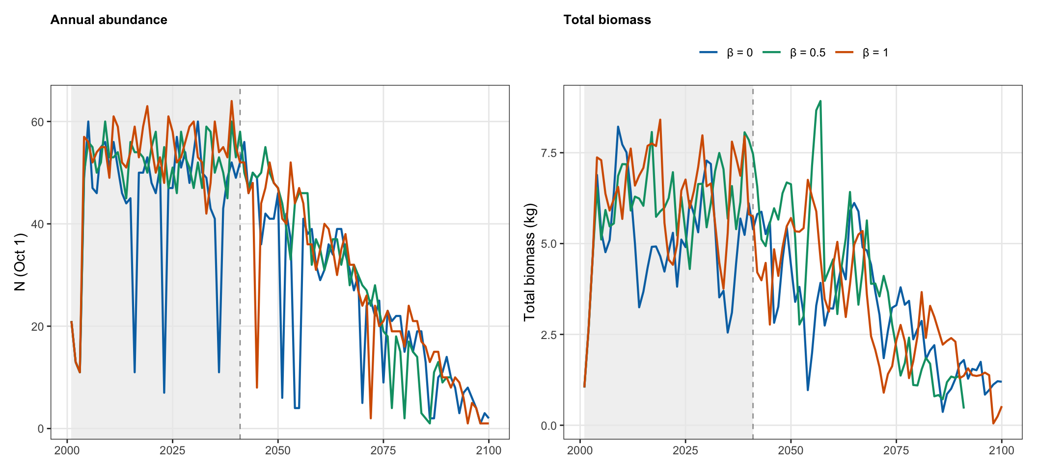
#| fig-cap: "Oct 1 annual abundance and total biomass for each dominance_beta value."
#| fig-height: 5
p_N <- ggplot(beta_census, aes(x = year, y = N, color = label)) +
  annotate("rect", xmin = burn_start, xmax = exp_start_yr,
           ymin = -Inf, ymax = Inf, fill = "grey92", alpha = 0.7) +
  geom_vline(xintercept = exp_start_yr, linetype = "dashed",
             color = "grey55", linewidth = 0.4) +
  geom_line(linewidth = 0.75) +
  scale_color_manual(values = beta_cols) +
  labs(x = NULL, y = "N (Oct 1)", color = NULL, title = "Annual abundance") +
  theme_sens() + theme(legend.position = "none")

p_B <- ggplot(beta_census, aes(x = year, y = biomass_kg, color = label)) +
  annotate("rect", xmin = burn_start, xmax = exp_start_yr,
           ymin = -Inf, ymax = Inf, fill = "grey92", alpha = 0.7) +
  geom_vline(xintercept = exp_start_yr, linetype = "dashed",
             color = "grey55", linewidth = 0.4) +
  geom_line(linewidth = 0.75) +
  scale_color_manual(values = beta_cols) +
  labs(x = NULL, y = "Total biomass (kg)", color = NULL, title = "Total biomass") +
  theme_sens()

p_N | p_B
```
### Compensatory dynamics
```{r}
#| label: fig-beta-comp
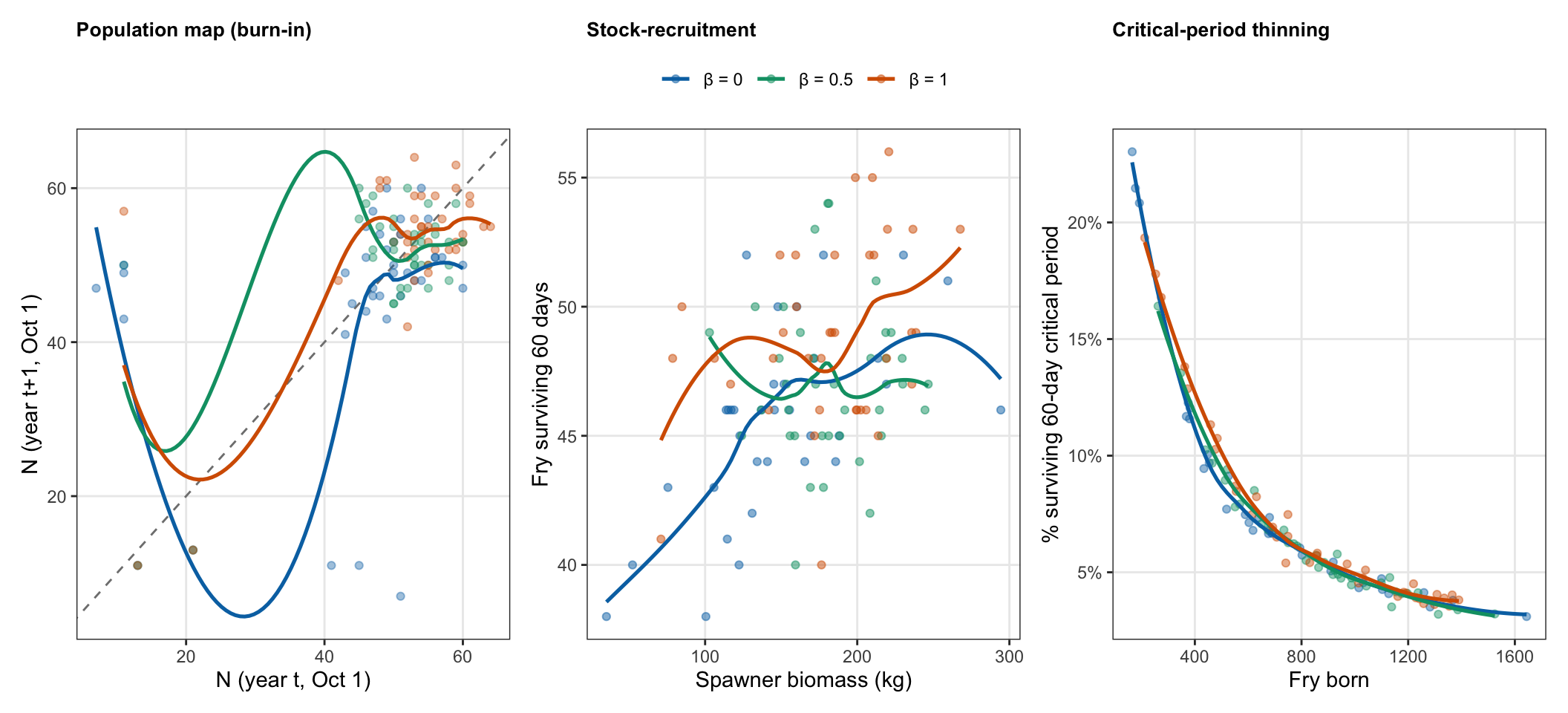
#| fig-cap: "Top-left: burn-in population map. Top-right: stock-recruitment. Bottom-left: size-based early thinning (% of fry surviving to day 60). Bottom-right: density–growth relationship. The bottom row together shows the two pathways of size-based density-dependent compensation: cohort thinning (left) and growth suppression (right)."
#| fig-height: 8
beta_map <- pop_map(beta_census)

p_map <- ggplot(beta_map, aes(x = N, y = N_next, color = label)) +
  geom_abline(slope = 1, intercept = 0, linetype = "dashed", color = "grey50") +
  geom_point(alpha = 0.4, size = 1.5) +
  geom_smooth(method = "loess", se = FALSE, span = 0.75, linewidth = 0.9) +
  scale_color_manual(values = beta_cols) +
  labs(x = "N (year t, Oct 1)", y = "N (year t+1, Oct 1)", color = NULL,
       title = "Population map (burn-in)") +
  theme_sens() + theme(legend.position = "none")

p_sr <- ggplot(beta_sr |> filter(spawner_kg > 0),
               aes(x = spawner_kg, y = bio_surv60_kg, color = label)) +
  geom_point(alpha = 0.5, size = 1.5) +
  geom_smooth(method = "loess", se = FALSE, span = 0.7, linewidth = 0.9) +
  scale_color_manual(values = beta_cols) +
  labs(x = "Spawner biomass (kg)", y = "Fry biomass at 60 days (kg)",
       color = NULL, title = "Stock-recruitment") +
  theme_sens() + theme(legend.position = "right")

p_thin <- ggplot(beta_thin, aes(x = n_born, y = surv_rate, color = label)) +
  geom_point(alpha = 0.45, size = 1.5) +
  geom_smooth(method = "loess", se = FALSE, span = 0.7, linewidth = 0.9) +
  scale_y_continuous(labels = scales::percent_format(accuracy = 1)) +
  scale_color_manual(values = beta_cols) +
  labs(x = "Fry born", y = "% of fry surviving to day 60",
       color = NULL, title = "Size-based thinning") +
  theme_sens() + theme(legend.position = "none")

p_dg <- ggplot(beta_dg, aes(x = mean_july_n, y = mean_wt, color = label)) +
  geom_point(alpha = 0.5, size = 1.5) +
  geom_smooth(method = "lm", se = FALSE, linewidth = 0.9) +
  geom_hline(yintercept = 7, linetype = "dotted", color = "grey50") +
  scale_color_manual(values = beta_cols) +
  labs(x = "Mean July N (all fish)", y = "Age-0 weight at Aug 1 (g)", color = NULL,
       title = "Density\u2013growth relationship",
       subtitle = "Higher density = slower early growth = more time below w\u2080") +
  theme_sens() + theme(legend.position = "none")

(p_map | p_sr) / (p_thin | p_dg)
```
### Age structure
```{r}
#| label: fig-beta-age0
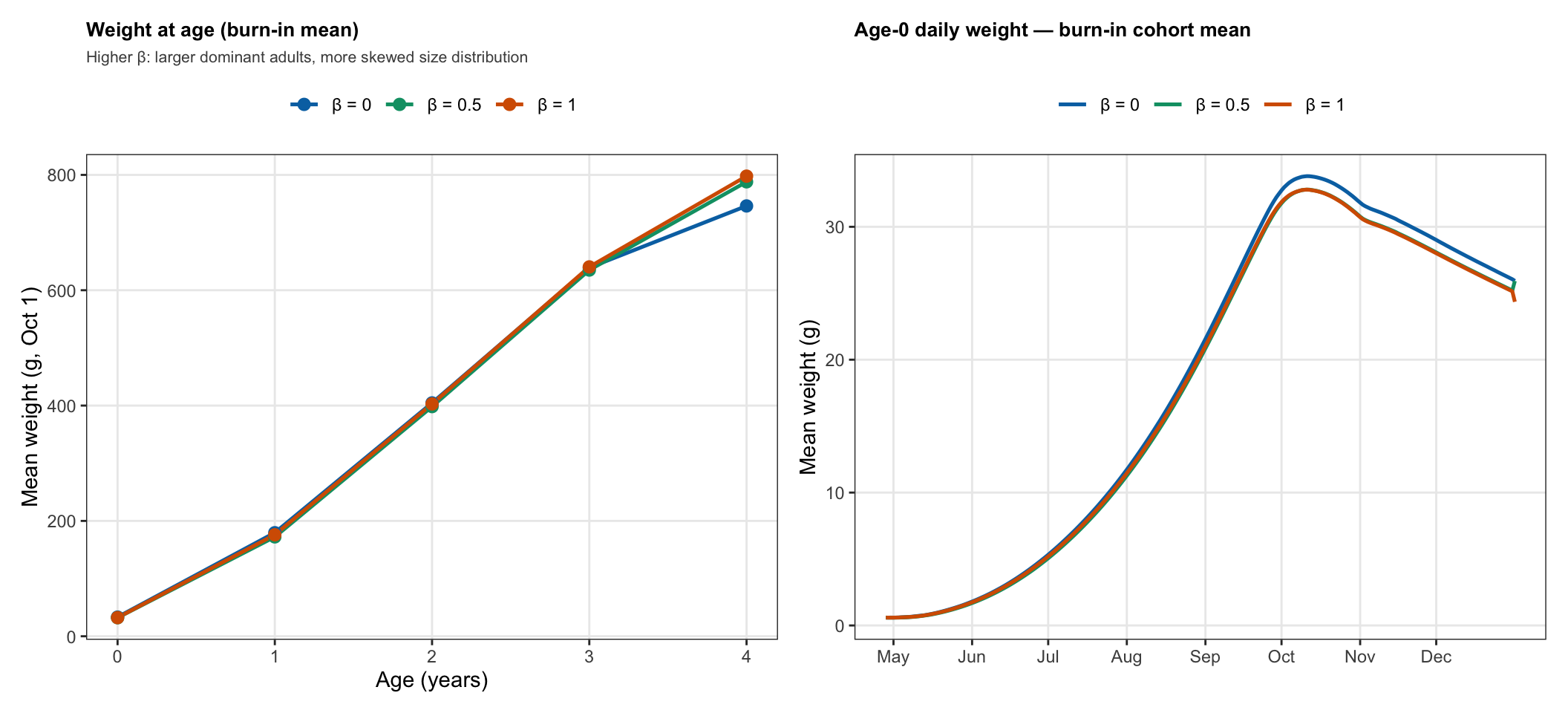
#| fig-cap: "Left: mean weight at age (burn-in). Right: age-0 daily weight by day of year, averaged across burn-in cohorts."
#| fig-height: 5
p_waa <- ggplot(beta_waa, aes(x = age_yrs, y = mean_wt, color = label)) +
  geom_line(linewidth = 0.9) +
  geom_point(size = 2.5) +
  scale_color_manual(values = beta_cols) +
  scale_x_continuous(breaks = 0:4) +
  labs(x = "Age (years)", y = "Mean weight (g, Oct 1)",
       color = NULL, title = "Weight at age (burn-in mean)",
       subtitle = "Higher β: larger dominant adults, more skewed size distribution") +
  theme_sens()

p_aget <- ggplot(beta_age0_dly |> filter(doy >= 118),
                 aes(x = doy, y = mean_wt, color = label)) +
  geom_line(linewidth = 0.9) +
  scale_color_manual(values = beta_cols) +
  scale_x_continuous(breaks = month_doys, labels = month_labels) +
  labs(x = NULL, y = "Mean weight (g)", color = NULL,
       title = "Age-0 daily weight — burn-in cohort mean") +
  theme_sens()

p_waa | p_aget
```
### Density-dependent duration below s_w0
```{r}
#| label: fig-beta-danger-duration
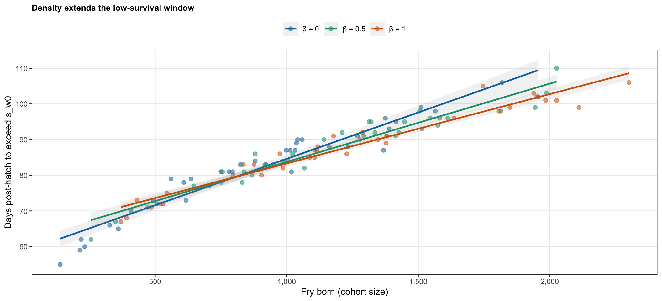
#| fig-cap: "Days post-hatch until cohort-mean weight first exceeds s_w0, vs fry born. Each point is one burn-in cohort year; lines are OLS fits with 95% CI."
#| fig-height: 5
beta_cross <- bind_rows(Map(days_to_threshold, beta_sims, beta_labels)) |>
  mutate(label = factor(label, levels = beta_labels))

plot_danger_duration(beta_cross, beta_cols)
```
### Stability summary {.unnumbered}
```{r}
#| label: fig-beta-stable
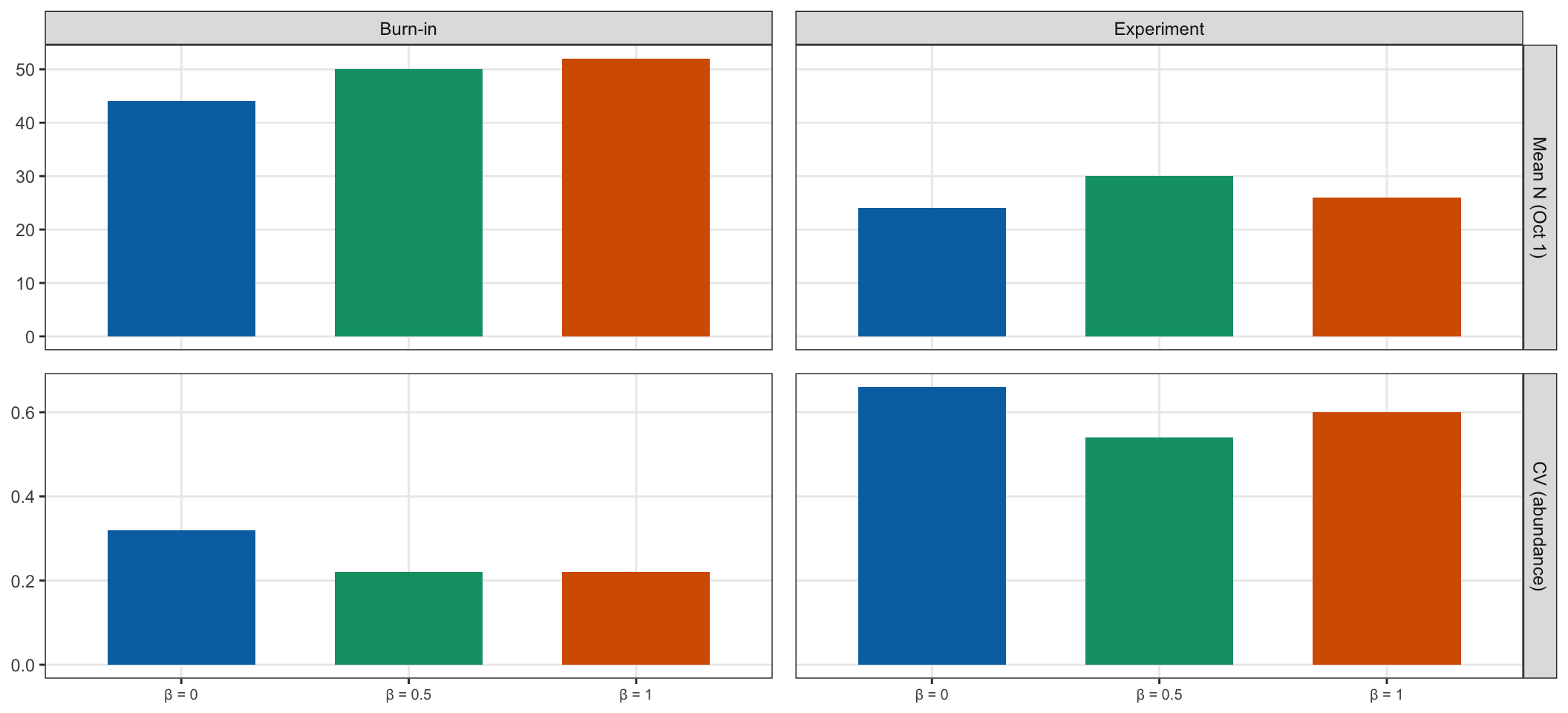
#| fig-cap: "Mean Oct 1 abundance and CV by dominance_beta, split by simulation phase."
#| fig-height: 5
plot_stability_fig(beta_stable, beta_cols)
```
```{r}
#| label: tbl-beta-stable
#| tbl-cap: "Stability statistics by dominance_beta."
beta_stable |>
  knitr::kable(col.names = c("β", "Phase", "Mean N",
                              "CV (abundance)", "Mean biomass (kg)", "Years"))
```
---
## `s_min`: size-survival floor (`minprob`)
`s_min` is the daily survival probability approached by the smallest fish (weight → 0).
It sets the intensity of early-life mortality for fish that have not yet grown past the
sigmoid inflection weight `s_w0`. Elliott (1993) reports ~6.4% daily mortality during
the early critical period for brown trout (`s_min ≈ 0.936`). Lower `s_min` strengthens
size-based thinning; higher `s_min` weakens it, reducing the compensatory effect of
density-dependent growth suppression.
| Scenario | `s_min` | Daily mortality floor | Worst-case 60-day survival at 0.5g |
|---|---|---|---|
| Low | 0.94 | 6% | 2.5% |
| **Baseline** | **0.96** | **4%** | **9%** |
| High | 0.98 | 2% | 30% |
All other parameters held at baseline.
```{r}
#| label: sim-s_min
#| cache: true
s_min_vals   <- c(0.94, 0.96, 0.98)
s_min_labels <- paste0("s_min = ", s_min_vals)
s_min_cols   <- sens_cols

cat("Running s_min sensitivity simulations...\n")
s_min_sims <- lapply(seq_along(s_min_vals), function(i) {
  cat(" s_min =", s_min_vals[i], "... ")
  p   <- modifyList(baseline, list(s_min = s_min_vals[i]))
  hdf <- build_habitat(p)
  res <- run_simulation(hdf, p, wt_growth = wt.growth)
  cat("ends", format(max(res$ibm_long$date, na.rm = TRUE)), "\n")
  res
})
names(s_min_sims) <- s_min_labels
```
```{r}
#| label: s_min-outcomes
s_min_census   <- bind_rows(Map(oct1_census,   s_min_sims, s_min_labels)) |>
  mutate(label = factor(label, levels = s_min_labels))
s_min_sr       <- bind_rows(Map(stock_recruit, s_min_sims, s_min_labels)) |>
  mutate(label = factor(label, levels = s_min_labels))
s_min_thin     <- bind_rows(Map(thinning_rate, s_min_sims, s_min_labels)) |>
  mutate(label = factor(label, levels = s_min_labels))
s_min_dg       <- bind_rows(Map(age0_density_growth, s_min_sims, s_min_labels)) |>
  mutate(label = factor(label, levels = s_min_labels))
s_min_waa      <- bind_rows(Map(wt_at_age, s_min_sims, s_min_labels)) |>
  mutate(label = factor(label, levels = s_min_labels))
s_min_age0_dly <- bind_rows(Map(age0_daily_wt, s_min_sims, s_min_labels)) |>
  mutate(label = factor(label, levels = s_min_labels))
s_min_stable   <- stability_stats(s_min_census)
```
### Abundance and biomass
```{r}
#| label: fig-s_min-ts
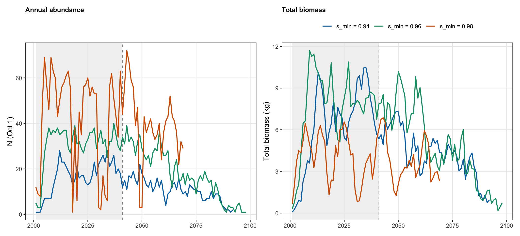
#| fig-cap: "Oct 1 annual abundance and total biomass for each s_min value."
#| fig-height: 5
p_N <- ggplot(s_min_census, aes(x = year, y = N, color = label)) +
  annotate("rect", xmin = burn_start, xmax = exp_start_yr,
           ymin = -Inf, ymax = Inf, fill = "grey92", alpha = 0.7) +
  geom_vline(xintercept = exp_start_yr, linetype = "dashed",
             color = "grey55", linewidth = 0.4) +
  geom_line(linewidth = 0.75) +
  scale_color_manual(values = s_min_cols) +
  labs(x = NULL, y = "N (Oct 1)", color = NULL, title = "Annual abundance") +
  theme_sens() + theme(legend.position = "none")

p_B <- ggplot(s_min_census, aes(x = year, y = biomass_kg, color = label)) +
  annotate("rect", xmin = burn_start, xmax = exp_start_yr,
           ymin = -Inf, ymax = Inf, fill = "grey92", alpha = 0.7) +
  geom_vline(xintercept = exp_start_yr, linetype = "dashed",
             color = "grey55", linewidth = 0.4) +
  geom_line(linewidth = 0.75) +
  scale_color_manual(values = s_min_cols) +
  labs(x = NULL, y = "Total biomass (kg)", color = NULL, title = "Total biomass") +
  theme_sens()

p_N | p_B
```
### Compensatory dynamics
```{r}
#| label: fig-s_min-comp
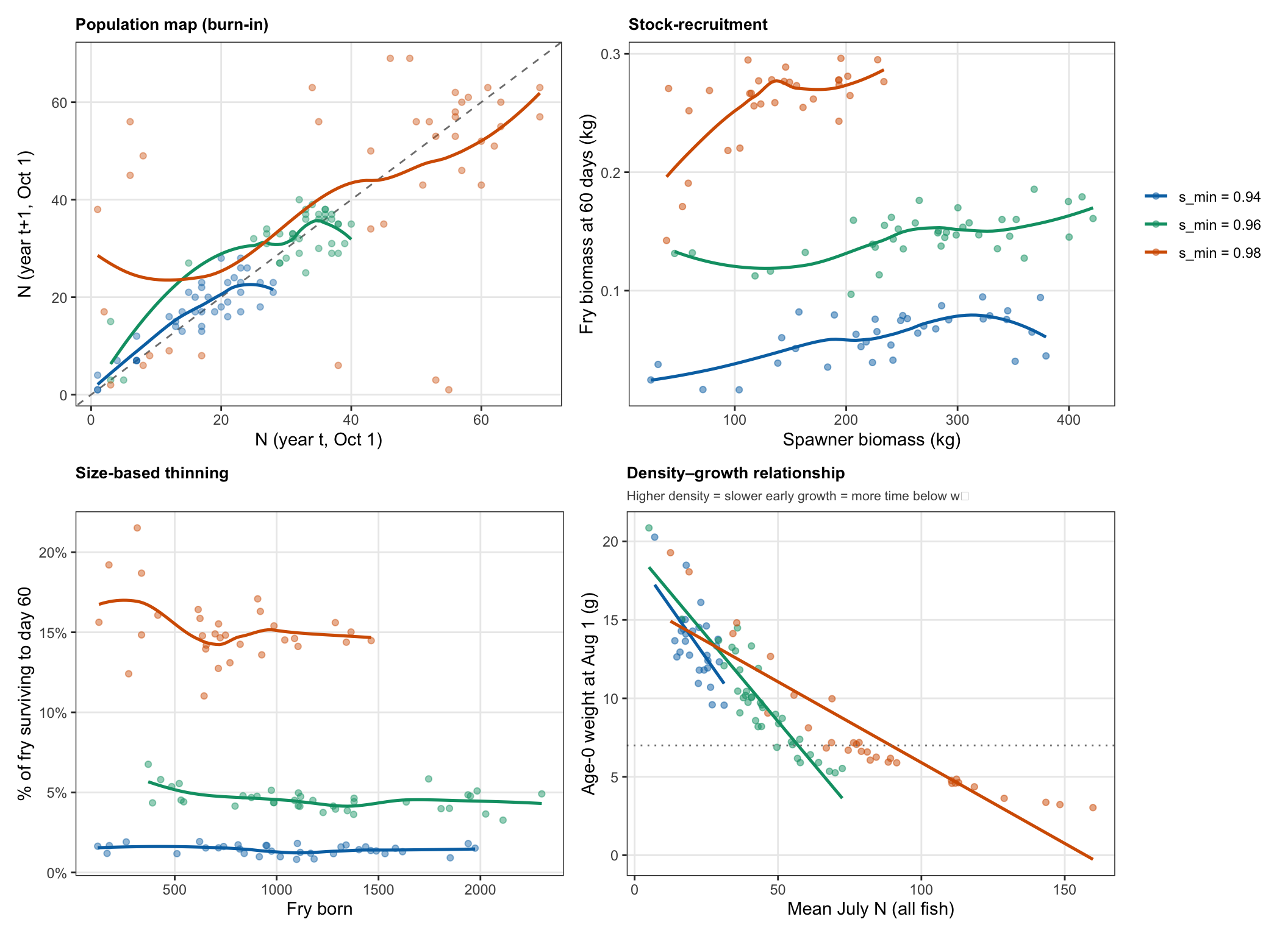
#| fig-cap: "Top-left: burn-in population map. Top-right: stock-recruitment. Bottom-left: size-based early thinning (% of fry surviving to day 60). Bottom-right: density–growth relationship. The bottom row together shows the two pathways of size-based density-dependent compensation: cohort thinning (left) and growth suppression (right)."
#| fig-height: 8
s_min_map <- pop_map(s_min_census)

p_map <- ggplot(s_min_map, aes(x = N, y = N_next, color = label)) +
  geom_abline(slope = 1, intercept = 0, linetype = "dashed", color = "grey50") +
  geom_point(alpha = 0.4, size = 1.5) +
  geom_smooth(method = "loess", se = FALSE, span = 0.75, linewidth = 0.9) +
  scale_color_manual(values = s_min_cols) +
  labs(x = "N (year t, Oct 1)", y = "N (year t+1, Oct 1)", color = NULL,
       title = "Population map (burn-in)") +
  theme_sens() + theme(legend.position = "none")

p_sr <- ggplot(s_min_sr |> filter(spawner_kg > 0),
               aes(x = spawner_kg, y = bio_surv60_kg, color = label)) +
  geom_point(alpha = 0.5, size = 1.5) +
  geom_smooth(method = "loess", se = FALSE, span = 0.7, linewidth = 0.9) +
  scale_color_manual(values = s_min_cols) +
  labs(x = "Spawner biomass (kg)", y = "Fry biomass at 60 days (kg)",
       color = NULL, title = "Stock-recruitment") +
  theme_sens() + theme(legend.position = "right")

p_thin <- ggplot(s_min_thin, aes(x = n_born, y = surv_rate, color = label)) +
  geom_point(alpha = 0.45, size = 1.5) +
  geom_smooth(method = "loess", se = FALSE, span = 0.7, linewidth = 0.9) +
  scale_y_continuous(labels = scales::percent_format(accuracy = 1)) +
  scale_color_manual(values = s_min_cols) +
  labs(x = "Fry born", y = "% of fry surviving to day 60",
       color = NULL, title = "Size-based thinning") +
  theme_sens() + theme(legend.position = "none")

p_dg <- ggplot(s_min_dg, aes(x = mean_july_n, y = mean_wt, color = label)) +
  geom_point(alpha = 0.5, size = 1.5) +
  geom_smooth(method = "lm", se = FALSE, linewidth = 0.9) +
  geom_hline(yintercept = 7, linetype = "dotted", color = "grey50") +
  scale_color_manual(values = s_min_cols) +
  labs(x = "Mean July N (all fish)", y = "Age-0 weight at Aug 1 (g)", color = NULL,
       title = "Density\u2013growth relationship",
       subtitle = "Higher density = slower early growth = more time below w\u2080") +
  theme_sens() + theme(legend.position = "none")

(p_map | p_sr) / (p_thin | p_dg)
```
### Age structure
```{r}
#| label: fig-s_min-age0
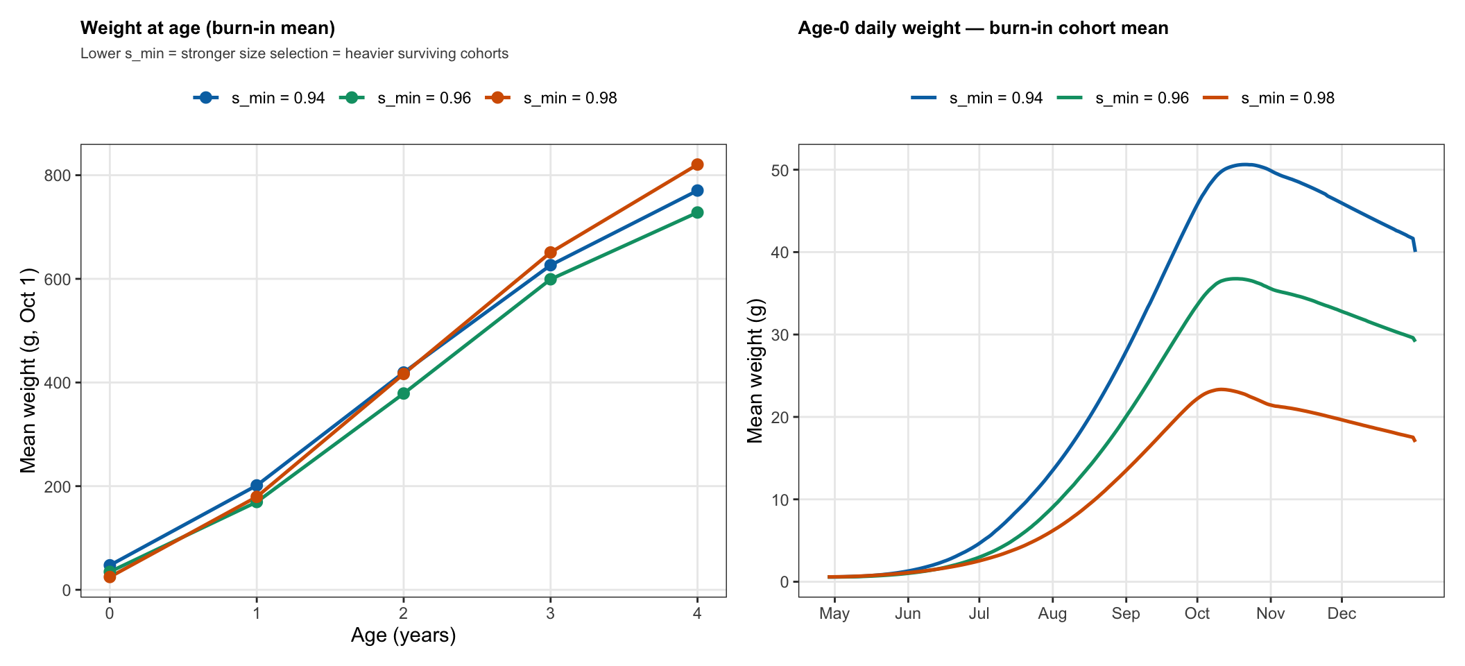
#| fig-cap: "Left: mean weight at age (burn-in). Right: age-0 daily weight by day of year, averaged across burn-in cohorts."
#| fig-height: 5
p_waa <- ggplot(s_min_waa, aes(x = age_yrs, y = mean_wt, color = label)) +
  geom_line(linewidth = 0.9) +
  geom_point(size = 2.5) +
  scale_color_manual(values = s_min_cols) +
  scale_x_continuous(breaks = 0:4) +
  labs(x = "Age (years)", y = "Mean weight (g, Oct 1)",
       color = NULL, title = "Weight at age (burn-in mean)",
       subtitle = "Lower s_min = stronger size selection = heavier surviving cohorts") +
  theme_sens()

p_aget <- ggplot(s_min_age0_dly |> filter(doy >= 118),
                 aes(x = doy, y = mean_wt, color = label)) +
  geom_line(linewidth = 0.9) +
  scale_color_manual(values = s_min_cols) +
  scale_x_continuous(breaks = month_doys, labels = month_labels) +
  labs(x = NULL, y = "Mean weight (g)", color = NULL,
       title = "Age-0 daily weight — burn-in cohort mean") +
  theme_sens()

p_waa | p_aget
```
### Density-dependent duration below s_w0
```{r}
#| label: fig-s_min-danger-duration
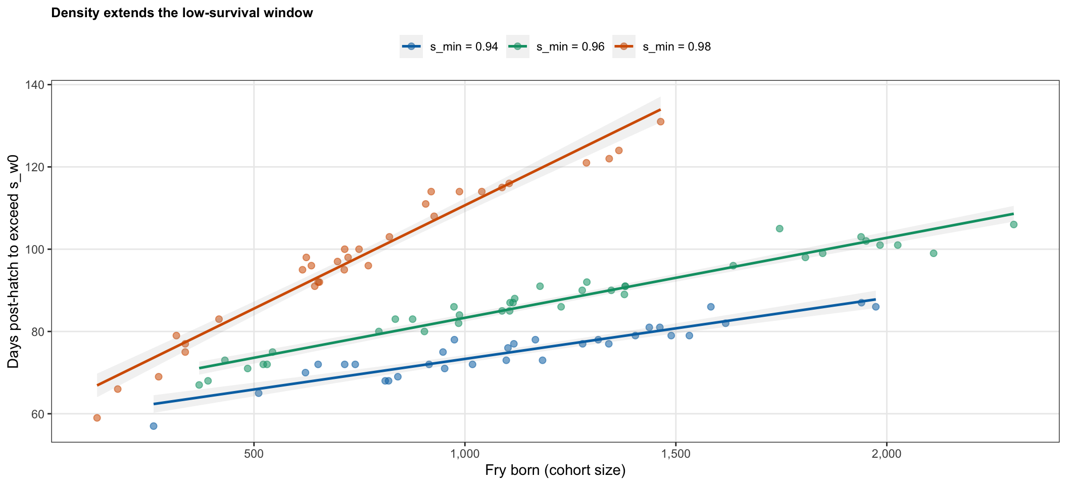
#| fig-cap: "Days post-hatch until cohort-mean weight first exceeds s_w0, vs fry born. Each point is one burn-in cohort year; lines are OLS fits with 95% CI."
#| fig-height: 5
s_min_cross <- bind_rows(Map(days_to_threshold, s_min_sims, s_min_labels)) |>
  mutate(label = factor(label, levels = s_min_labels))

plot_danger_duration(s_min_cross, s_min_cols)
```
### Stability summary {.unnumbered}
```{r}
#| label: fig-s_min-stable
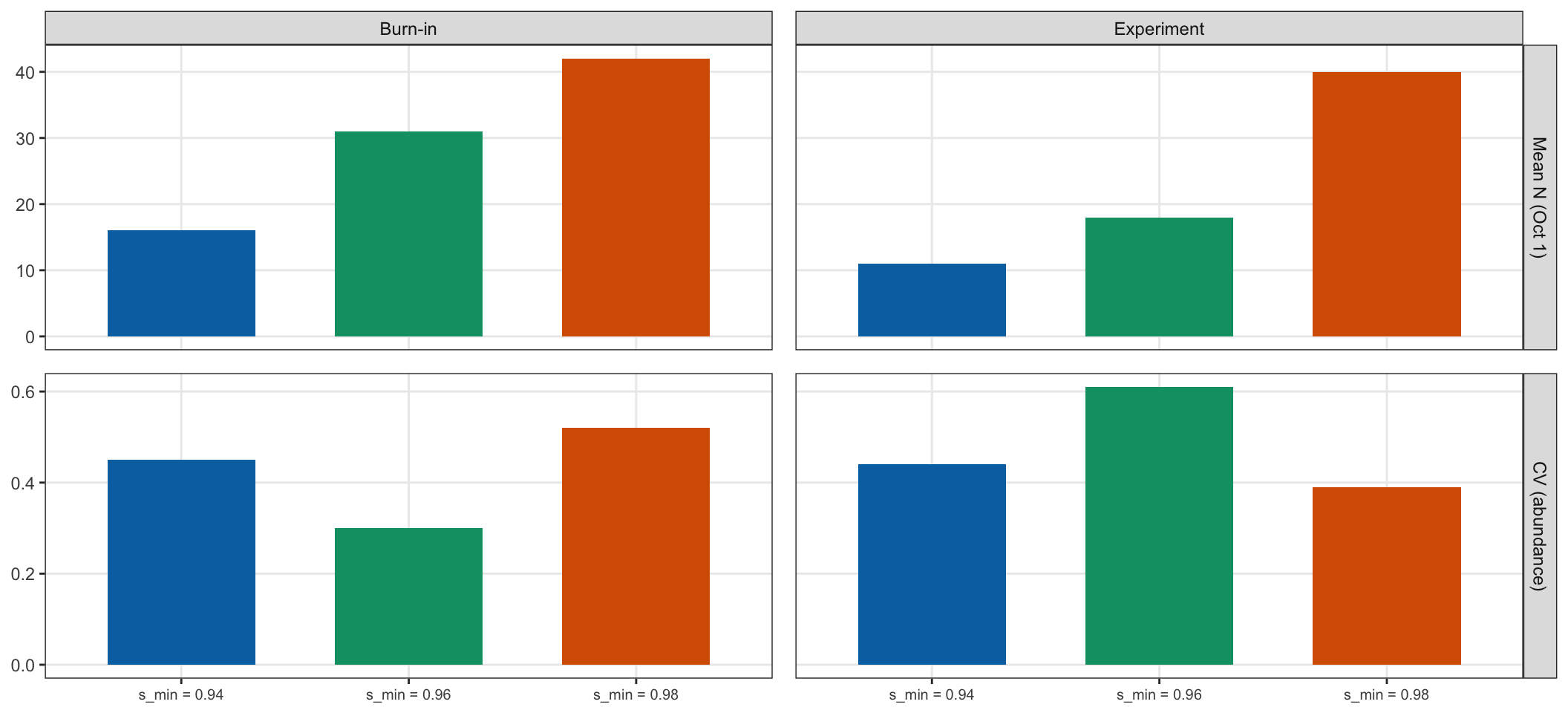
#| fig-cap: "Mean Oct 1 abundance and CV by s_min value, split by simulation phase."
#| fig-height: 5
plot_stability_fig(s_min_stable, s_min_cols)
```
```{r}
#| label: tbl-s_min-stable
#| tbl-cap: "Stability statistics by s_min value."
s_min_stable |>
  knitr::kable(col.names = c("s_min", "Phase", "Mean N",
                              "CV (abundance)", "Mean biomass (kg)", "Years"))
```
---
## `s_w0`: size-survival inflection weight
`s_w0` is the fish weight (g) at which daily survival is halfway between `s_min` and the
habitat-specific maximum. It defines how long fish remain in the high-mortality zone after
hatching: smaller `s_w0` means fish exit the danger zone sooner; larger `s_w0` prolongs
exposure. Based on visual inspection of age-0 daily weight trajectory plots, ~7g
corresponds to approximately 60 days post-hatch in cold habitat — the ecological basis
for the default. This section tests sensitivity to that assumption.
| Scenario | `s_w0` | Approx. days post-hatch to reach inflection (cold) |
|---|---|---|
| Low | 4g | ~35 days |
| **Baseline** | **7g** | **~60 days** |
| High | 10g | ~90 days |
All other parameters held at baseline.
```{r}
#| label: sim-s_w0
#| cache: true
w0_vals   <- c(4, 7, 10)
w0_labels <- paste0("s_w0 = ", w0_vals, "g")
w0_cols   <- sens_cols

cat("Running s_w0 sensitivity simulations...\n")
w0_sims <- lapply(seq_along(w0_vals), function(i) {
  cat(" s_w0 =", w0_vals[i], "... ")
  p   <- modifyList(baseline, list(s_w0 = w0_vals[i]))
  hdf <- build_habitat(p)
  res <- run_simulation(hdf, p, wt_growth = wt.growth)
  cat("ends", format(max(res$ibm_long$date, na.rm = TRUE)), "\n")
  res
})
names(w0_sims) <- w0_labels
```
```{r}
#| label: w0-outcomes
w0_census   <- bind_rows(Map(oct1_census,         w0_sims, w0_labels)) |>
  mutate(label = factor(label, levels = w0_labels))
w0_sr       <- bind_rows(Map(stock_recruit,       w0_sims, w0_labels)) |>
  mutate(label = factor(label, levels = w0_labels))
w0_thin     <- bind_rows(Map(thinning_rate,       w0_sims, w0_labels)) |>
  mutate(label = factor(label, levels = w0_labels))
w0_dg       <- bind_rows(Map(age0_density_growth, w0_sims, w0_labels)) |>
  mutate(label = factor(label, levels = w0_labels))
w0_waa      <- bind_rows(Map(wt_at_age,           w0_sims, w0_labels)) |>
  mutate(label = factor(label, levels = w0_labels))
w0_age0_dly <- bind_rows(Map(age0_daily_wt,       w0_sims, w0_labels)) |>
  mutate(label = factor(label, levels = w0_labels))
w0_stable   <- stability_stats(w0_census)
```
### Abundance and biomass
```{r}
#| label: fig-w0-ts
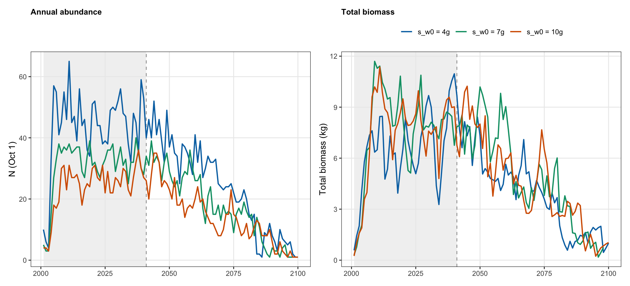
#| fig-cap: "Oct 1 annual abundance and total biomass for each s_w0 value. Grey band = burn-in."
#| fig-height: 5
p_N <- ggplot(w0_census, aes(x = year, y = N, color = label)) +
  annotate("rect", xmin = burn_start, xmax = exp_start_yr,
           ymin = -Inf, ymax = Inf, fill = "grey92", alpha = 0.7) +
  geom_vline(xintercept = exp_start_yr, linetype = "dashed",
             color = "grey55", linewidth = 0.4) +
  geom_line(linewidth = 0.75) +
  scale_color_manual(values = w0_cols) +
  labs(x = NULL, y = "N (Oct 1)", color = NULL, title = "Annual abundance") +
  theme_sens() + theme(legend.position = "none")

p_B <- ggplot(w0_census, aes(x = year, y = biomass_kg, color = label)) +
  annotate("rect", xmin = burn_start, xmax = exp_start_yr,
           ymin = -Inf, ymax = Inf, fill = "grey92", alpha = 0.7) +
  geom_vline(xintercept = exp_start_yr, linetype = "dashed",
             color = "grey55", linewidth = 0.4) +
  geom_line(linewidth = 0.75) +
  scale_color_manual(values = w0_cols) +
  labs(x = NULL, y = "Total biomass (kg)", color = NULL, title = "Total biomass") +
  theme_sens()

p_N | p_B
```
### Compensatory dynamics
```{r}
#| label: fig-w0-comp
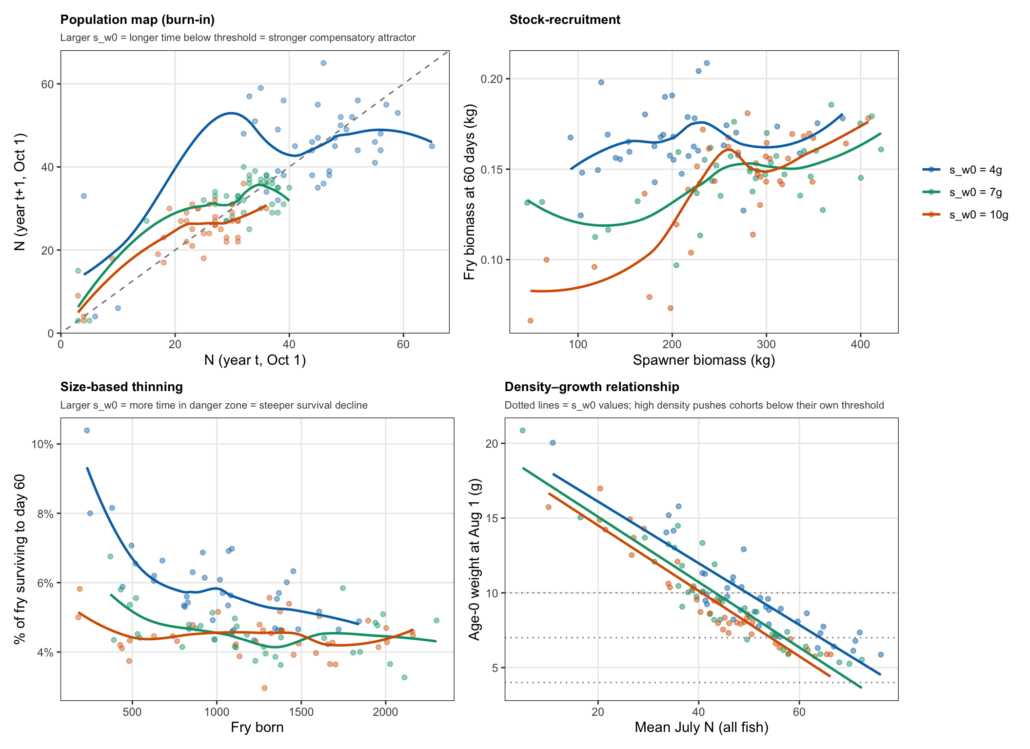
#| fig-cap: "Top-left: burn-in population map. Top-right: stock-recruitment. Bottom-left: size-based early thinning (% of fry surviving to day 60). Bottom-right: density–growth relationship. The bottom row together shows the two pathways of size-based density-dependent compensation: cohort thinning (left) and growth suppression (right). Dotted lines in the density–growth panel mark the three s_w0 values tested."
#| fig-height: 8
w0_map <- pop_map(w0_census)

p_map <- ggplot(w0_map, aes(x = N, y = N_next, color = label)) +
  geom_abline(slope = 1, intercept = 0, linetype = "dashed", color = "grey50") +
  geom_point(alpha = 0.4, size = 1.5) +
  geom_smooth(method = "loess", se = FALSE, span = 0.75, linewidth = 0.9) +
  scale_color_manual(values = w0_cols) +
  labs(x = "N (year t, Oct 1)", y = "N (year t+1, Oct 1)", color = NULL,
       title = "Population map (burn-in)",
       subtitle = "Larger s_w0 = longer time below threshold = stronger compensatory attractor") +
  theme_sens() + theme(legend.position = "none")

p_sr <- ggplot(w0_sr |> filter(spawner_kg > 0),
               aes(x = spawner_kg, y = bio_surv60_kg, color = label)) +
  geom_point(alpha = 0.5, size = 1.5) +
  geom_smooth(method = "loess", se = FALSE, span = 0.7, linewidth = 0.9) +
  scale_color_manual(values = w0_cols) +
  labs(x = "Spawner biomass (kg)", y = "Fry biomass at 60 days (kg)",
       color = NULL, title = "Stock-recruitment") +
  theme_sens() + theme(legend.position = "right")

p_thin <- ggplot(w0_thin, aes(x = n_born, y = surv_rate, color = label)) +
  geom_point(alpha = 0.45, size = 1.5) +
  geom_smooth(method = "loess", se = FALSE, span = 0.7, linewidth = 0.9) +
  scale_y_continuous(labels = scales::percent_format(accuracy = 1)) +
  scale_color_manual(values = w0_cols) +
  labs(x = "Fry born", y = "% of fry surviving to day 60",
       color = NULL, title = "Size-based thinning",
       subtitle = "Larger s_w0 = more time in danger zone = steeper survival decline") +
  theme_sens() + theme(legend.position = "none")

p_dg <- ggplot(w0_dg, aes(x = mean_july_n, y = mean_wt, color = label)) +
  geom_point(alpha = 0.5, size = 1.5) +
  geom_smooth(method = "lm", se = FALSE, linewidth = 0.9) +
  geom_hline(yintercept = c(4, 7, 10), linetype = "dotted", color = "grey50") +
  scale_color_manual(values = w0_cols) +
  labs(x = "Mean July N (all fish)", y = "Age-0 weight at Aug 1 (g)", color = NULL,
       title = "Density\u2013growth relationship",
       subtitle = "Dotted lines = s_w0 values; high density pushes cohorts below their own threshold") +
  theme_sens() + theme(legend.position = "none")

(p_map | p_sr) / (p_thin | p_dg)
```
### Age structure
```{r}
#| label: fig-w0-age0
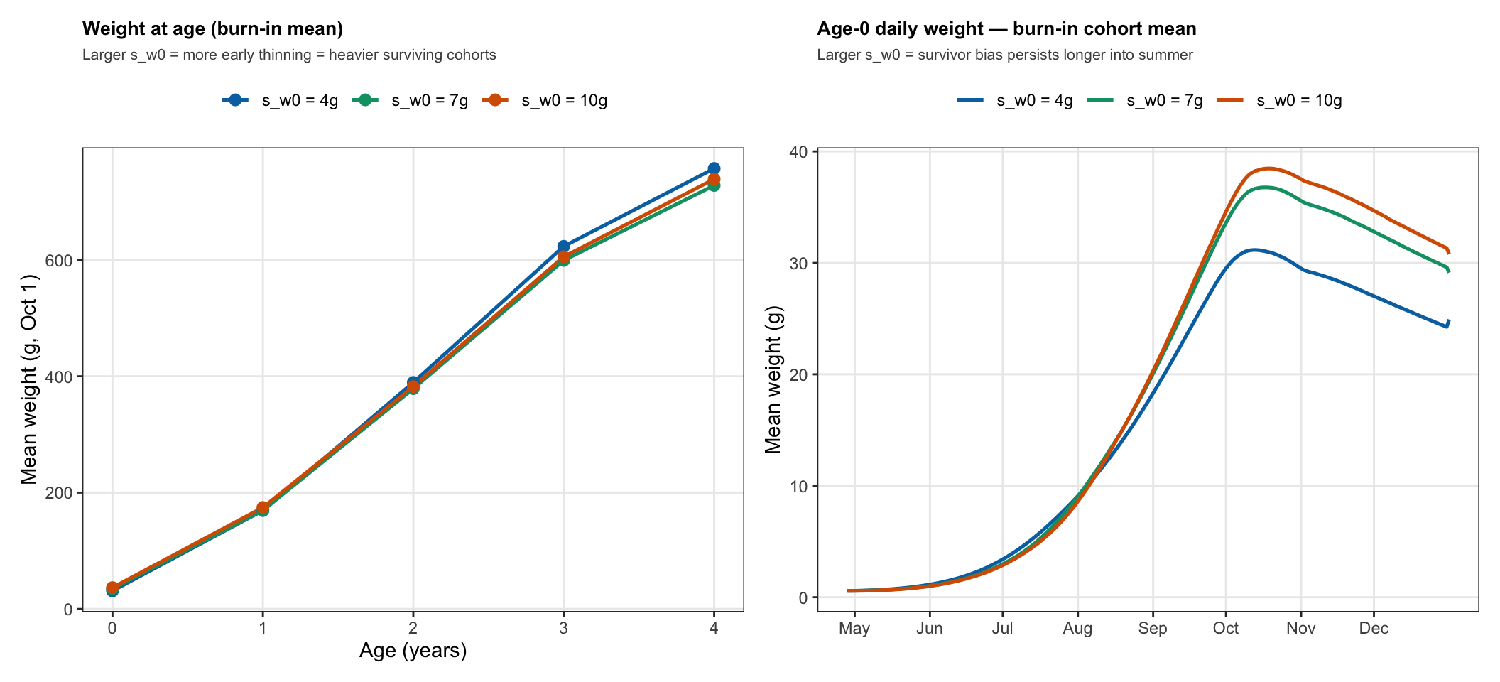
#| fig-cap: "Left: mean weight at age (burn-in). Right: age-0 daily weight by day of year, averaged across burn-in cohorts."
#| fig-height: 5
p_waa <- ggplot(w0_waa, aes(x = age_yrs, y = mean_wt, color = label)) +
  geom_line(linewidth = 0.9) +
  geom_point(size = 2.5) +
  scale_color_manual(values = w0_cols) +
  scale_x_continuous(breaks = 0:4) +
  labs(x = "Age (years)", y = "Mean weight (g, Oct 1)",
       color = NULL, title = "Weight at age (burn-in mean)",
       subtitle = "Larger s_w0 = more early thinning = heavier surviving cohorts") +
  theme_sens()

p_aget <- ggplot(w0_age0_dly |> filter(doy >= 118),
                 aes(x = doy, y = mean_wt, color = label)) +
  geom_line(linewidth = 0.9) +
  scale_color_manual(values = w0_cols) +
  scale_x_continuous(breaks = month_doys, labels = month_labels) +
  labs(x = NULL, y = "Mean weight (g)", color = NULL,
       title = "Age-0 daily weight \u2014 burn-in cohort mean",
       subtitle = "Larger s_w0 = survivor bias persists longer into summer") +
  theme_sens()

p_waa | p_aget
```
### Density-dependent duration below s_w0
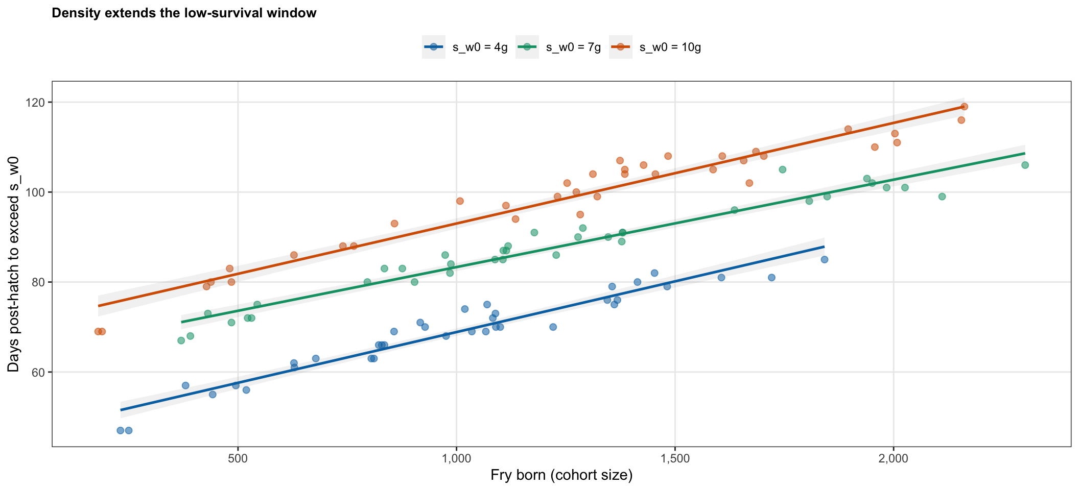
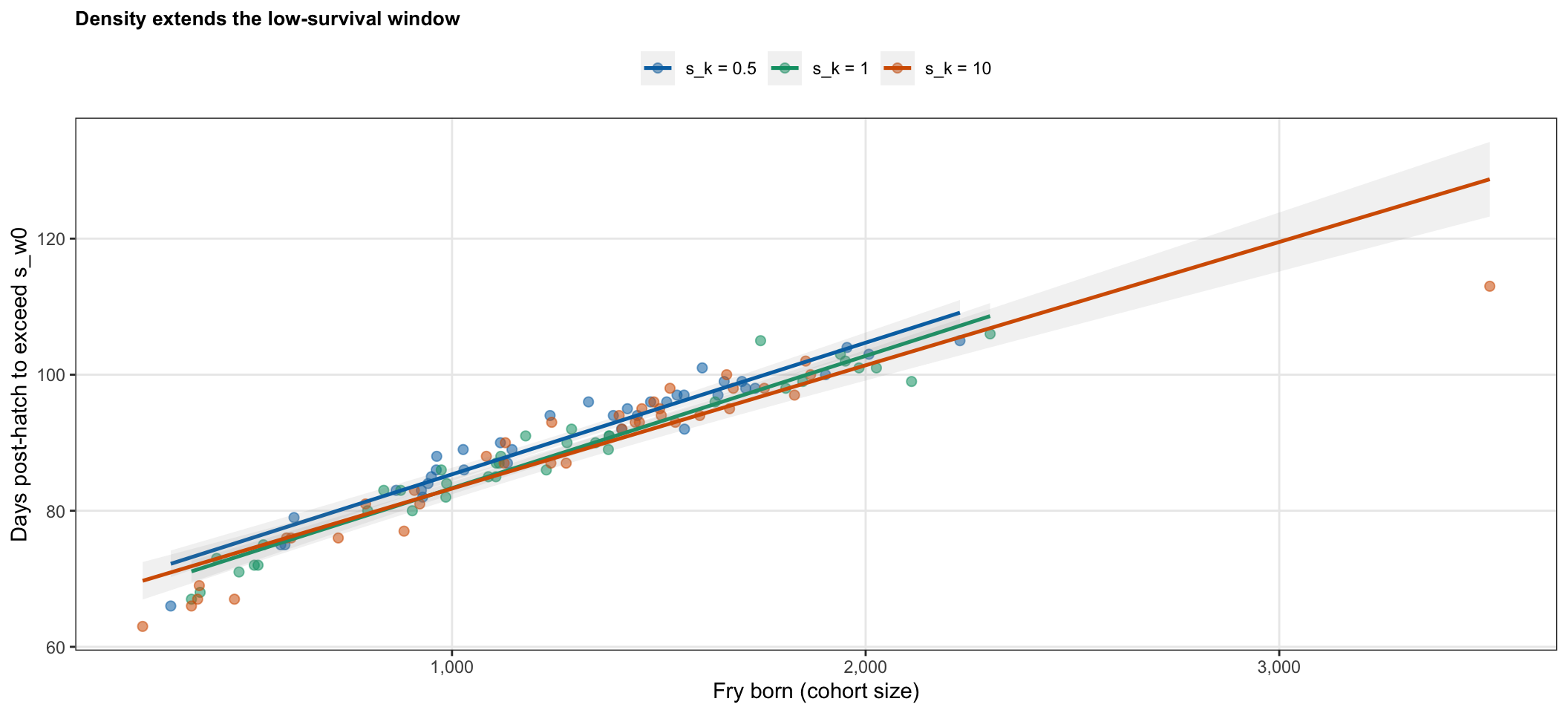
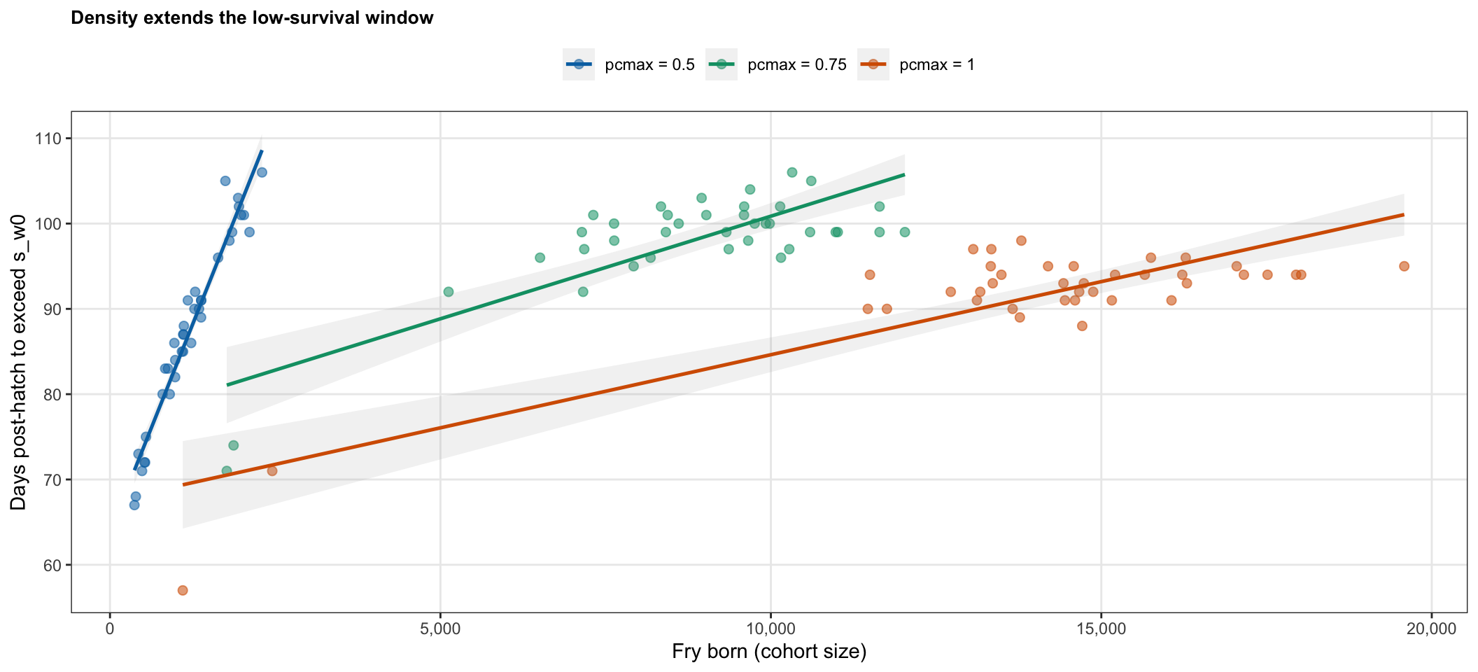
Larger cohorts experience slower growth through food competition, which delays
the date at which mean cohort weight first exceeds `s_w0`. This plot directly
quantifies that effect: the x-axis is cohort size (fry born), the y-axis is
days post-hatch until the burn-in cohort-mean weight trajectory first crosses
`s_w0`. A positive slope confirms that density extends the low-survival window,
and the slope magnitude indicates how many extra days of size-based mortality
each additional 1,000 fry born imposes.
`n_born` is used as the density metric because it is causally prior — it is the
initial condition that drives food competition. An alternative is age-0 abundance
in early June (the competitive environment fish actually experience), but in
practice this is highly correlated with `n_born` and harder to extract.
```{r}
#| label: fig-w0-danger-duration
#| fig-cap: "Days post-hatch until the burn-in cohort-mean weight first exceeds s_w0, plotted against cohort size (fry born). Each point is one burn-in cohort year. Lines are OLS fits with 95% CI. The near-identical slopes across s_w0 values indicate that the density-dependent extension of the low-survival window (~20 extra days per 1,000 fry born) is a property of the growth response to density, not the threshold level."
#| fig-height: 5
w0_cross <- bind_rows(Map(days_to_threshold, w0_sims, w0_labels)) |>
  mutate(label = factor(label, levels = w0_labels))

plot_danger_duration(w0_cross, w0_cols)
```
### Stability summary {.unnumbered}
```{r}
#| label: fig-w0-stable
#| fig-cap: "Mean Oct 1 abundance and CV by s_w0 value, split by simulation phase."
#| fig-height: 5
plot_stability_fig(w0_stable, w0_cols)
```
```{r}
#| label: tbl-w0-stable
#| tbl-cap: "Stability statistics by s_w0 value."
w0_stable |>
  knitr::kable(col.names = c("s_w0", "Phase", "Mean N",
                              "CV (abundance)", "Mean biomass (kg)", "Years"))
```
---
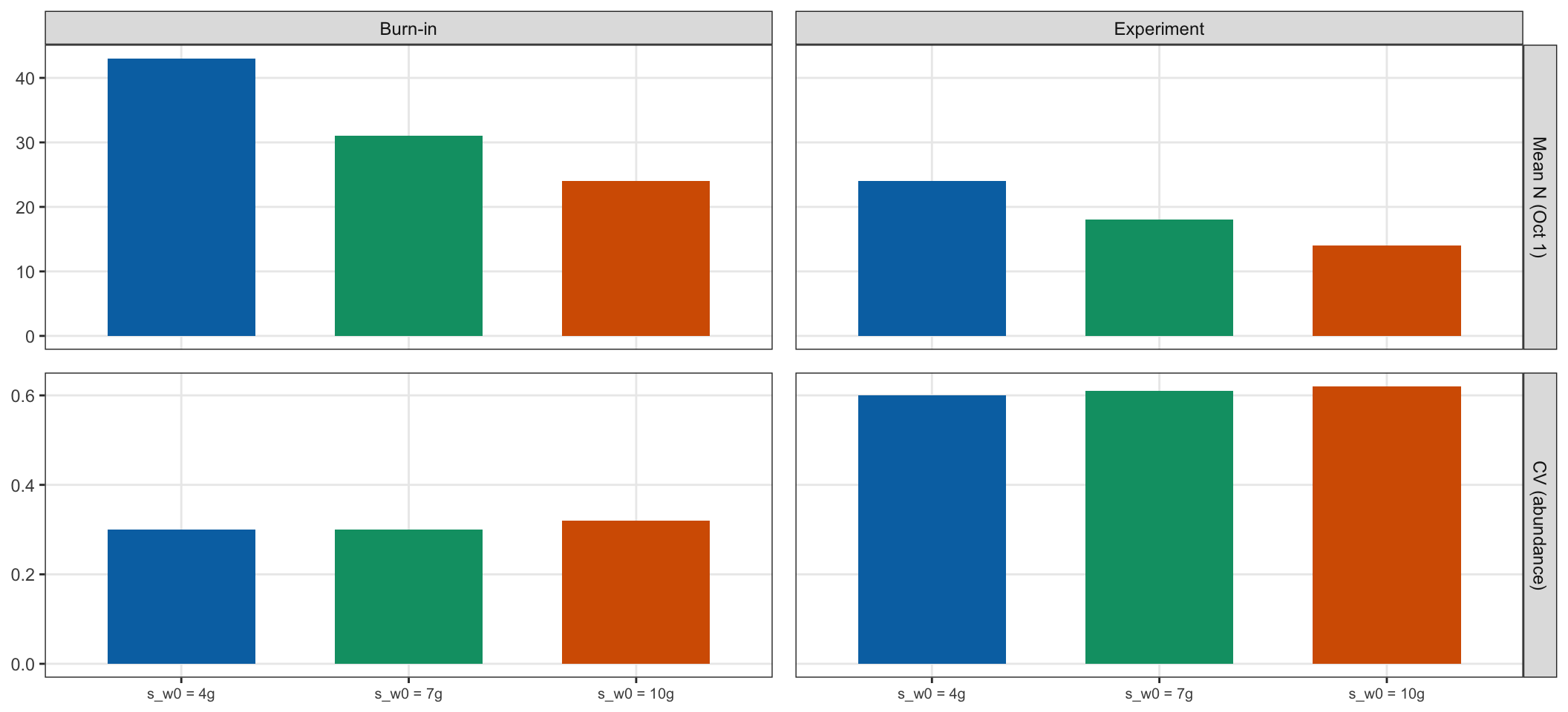
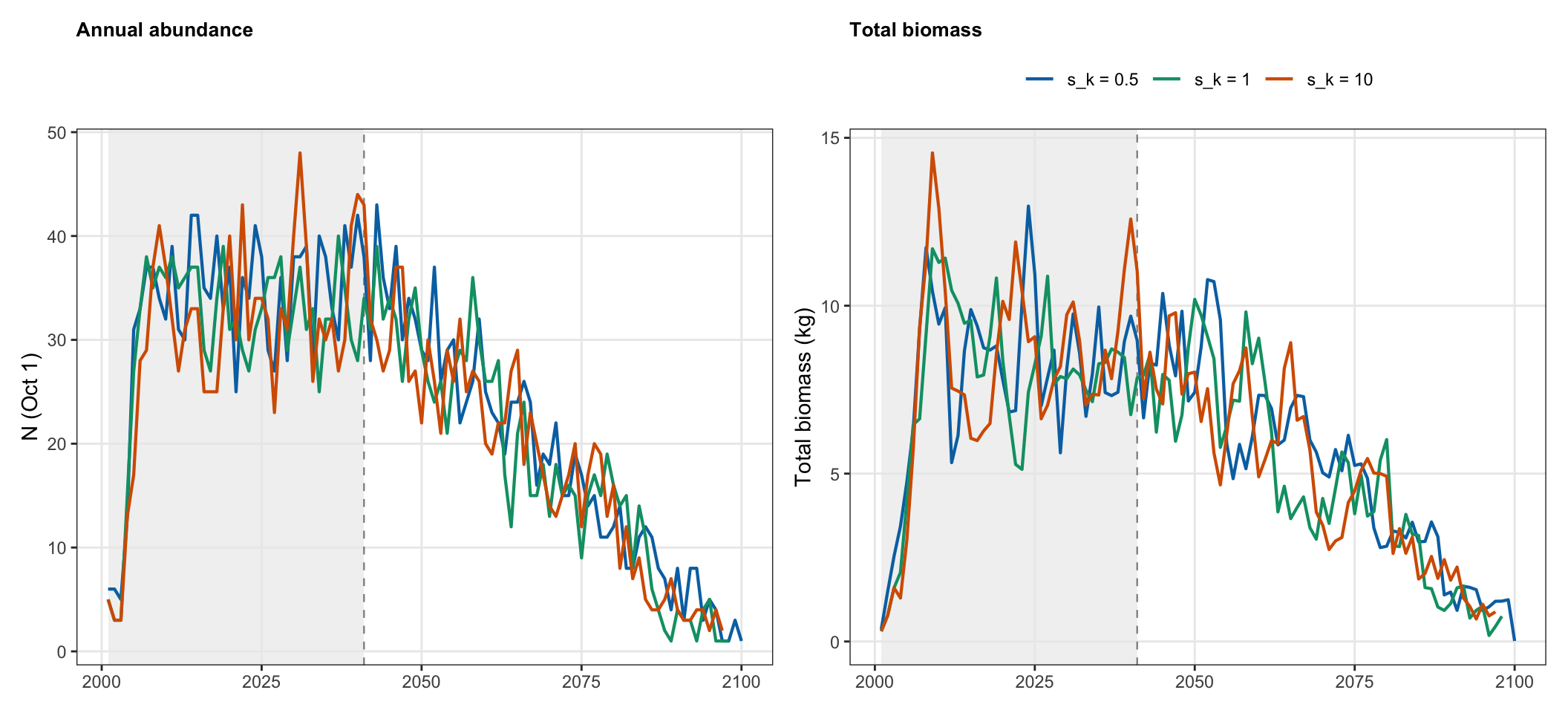
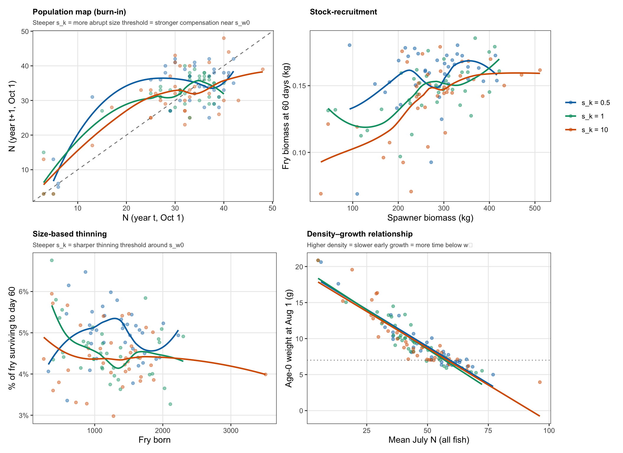
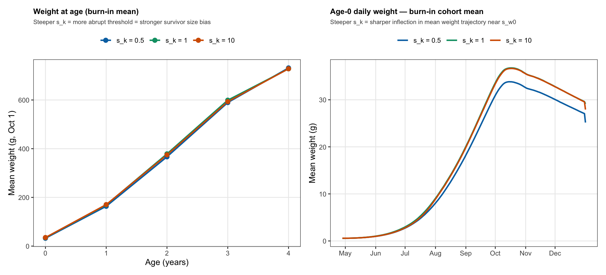
## `s_k`: sigmoid steepness
`s_k` controls how sharply daily survival transitions from `s_min` to the habitat-specific
maximum near `s_w0`. Low `s_k` produces a gradual transition spread across a wide size
range; high `s_k` creates a near-cliff where fish below `s_w0` experience near-`s_min`
mortality and fish above it experience near-maximum survival. The transition width from
10% to 90% of the full `s_min`–`s_max` range spans w₀ ± ln(9)/s_k grams.
| Scenario | `s_k` | Transition width (10%–90% of range) | Character |
|---|---|---|---|
| Shallow | 0.5 | ±4.4g around `s_w0` | Gradual — broad size range under partial penalty |
| **Baseline** | **1** | **±2.2g around `s_w0`** | **Moderate transition** |
| Steep | 10 | ±0.2g around `s_w0` | Near-cliff — survival almost binary at `s_w0` |
All other parameters held at baseline.
```{r}
#| label: sim-s_k
#| cache: true
sk_vals   <- c(0.5, 1, 10)
sk_labels <- paste0("s_k = ", sk_vals)
sk_cols   <- sens_cols

cat("Running s_k sensitivity simulations...\n")
sk_sims <- lapply(seq_along(sk_vals), function(i) {
  cat(" s_k =", sk_vals[i], "... ")
  p   <- modifyList(baseline, list(s_k = sk_vals[i]))
  hdf <- build_habitat(p)
  res <- run_simulation(hdf, p, wt_growth = wt.growth)
  cat("ends", format(max(res$ibm_long$date, na.rm = TRUE)), "\n")
  res
})
names(sk_sims) <- sk_labels
```
```{r}
#| label: sk-outcomes
sk_census   <- bind_rows(Map(oct1_census,         sk_sims, sk_labels)) |>
  mutate(label = factor(label, levels = sk_labels))
sk_sr       <- bind_rows(Map(stock_recruit,       sk_sims, sk_labels)) |>
  mutate(label = factor(label, levels = sk_labels))
sk_thin     <- bind_rows(Map(thinning_rate,       sk_sims, sk_labels)) |>
  mutate(label = factor(label, levels = sk_labels))
sk_dg       <- bind_rows(Map(age0_density_growth, sk_sims, sk_labels)) |>
  mutate(label = factor(label, levels = sk_labels))
sk_waa      <- bind_rows(Map(wt_at_age,           sk_sims, sk_labels)) |>
  mutate(label = factor(label, levels = sk_labels))
sk_age0_dly <- bind_rows(Map(age0_daily_wt,       sk_sims, sk_labels)) |>
  mutate(label = factor(label, levels = sk_labels))
sk_stable   <- stability_stats(sk_census)
```
### Abundance and biomass
```{r}
#| label: fig-sk-ts
#| fig-cap: "Oct 1 annual abundance and total biomass for each s_k value. Grey band = burn-in."
#| fig-height: 5
p_N <- ggplot(sk_census, aes(x = year, y = N, color = label)) +
  annotate("rect", xmin = burn_start, xmax = exp_start_yr,
           ymin = -Inf, ymax = Inf, fill = "grey92", alpha = 0.7) +
  geom_vline(xintercept = exp_start_yr, linetype = "dashed",
             color = "grey55", linewidth = 0.4) +
  geom_line(linewidth = 0.75) +
  scale_color_manual(values = sk_cols) +
  labs(x = NULL, y = "N (Oct 1)", color = NULL, title = "Annual abundance") +
  theme_sens() + theme(legend.position = "none")

p_B <- ggplot(sk_census, aes(x = year, y = biomass_kg, color = label)) +
  annotate("rect", xmin = burn_start, xmax = exp_start_yr,
           ymin = -Inf, ymax = Inf, fill = "grey92", alpha = 0.7) +
  geom_vline(xintercept = exp_start_yr, linetype = "dashed",
             color = "grey55", linewidth = 0.4) +
  geom_line(linewidth = 0.75) +
  scale_color_manual(values = sk_cols) +
  labs(x = NULL, y = "Total biomass (kg)", color = NULL, title = "Total biomass") +
  theme_sens()

p_N | p_B
```
### Compensatory dynamics
```{r}
#| label: fig-sk-comp
#| fig-cap: "Top-left: burn-in population map. Top-right: stock-recruitment. Bottom-left: size-based early thinning (% of fry surviving to day 60). Bottom-right: density–growth relationship. The bottom row together shows the two pathways of size-based density-dependent compensation: cohort thinning (left) and growth suppression (right)."
#| fig-height: 8
sk_map <- pop_map(sk_census)

p_map <- ggplot(sk_map, aes(x = N, y = N_next, color = label)) +
  geom_abline(slope = 1, intercept = 0, linetype = "dashed", color = "grey50") +
  geom_point(alpha = 0.4, size = 1.5) +
  geom_smooth(method = "loess", se = FALSE, span = 0.75, linewidth = 0.9) +
  scale_color_manual(values = sk_cols) +
  labs(x = "N (year t, Oct 1)", y = "N (year t+1, Oct 1)", color = NULL,
       title = "Population map (burn-in)",
       subtitle = "Steeper s_k = more abrupt size threshold = stronger compensation near s_w0") +
  theme_sens() + theme(legend.position = "none")

p_sr <- ggplot(sk_sr |> filter(spawner_kg > 0),
               aes(x = spawner_kg, y = bio_surv60_kg, color = label)) +
  geom_point(alpha = 0.5, size = 1.5) +
  geom_smooth(method = "loess", se = FALSE, span = 0.7, linewidth = 0.9) +
  scale_color_manual(values = sk_cols) +
  labs(x = "Spawner biomass (kg)", y = "Fry biomass at 60 days (kg)",
       color = NULL, title = "Stock-recruitment") +
  theme_sens() + theme(legend.position = "right")

p_thin <- ggplot(sk_thin, aes(x = n_born, y = surv_rate, color = label)) +
  geom_point(alpha = 0.45, size = 1.5) +
  geom_smooth(method = "loess", se = FALSE, span = 0.7, linewidth = 0.9) +
  scale_y_continuous(labels = scales::percent_format(accuracy = 1)) +
  scale_color_manual(values = sk_cols) +
  labs(x = "Fry born", y = "% of fry surviving to day 60",
       color = NULL, title = "Size-based thinning",
       subtitle = "Steeper s_k = sharper thinning threshold around s_w0") +
  theme_sens() + theme(legend.position = "none")

p_dg <- ggplot(sk_dg, aes(x = mean_july_n, y = mean_wt, color = label)) +
  geom_point(alpha = 0.5, size = 1.5) +
  geom_smooth(method = "lm", se = FALSE, linewidth = 0.9) +
  geom_hline(yintercept = 7, linetype = "dotted", color = "grey50") +
  scale_color_manual(values = sk_cols) +
  labs(x = "Mean July N (all fish)", y = "Age-0 weight at Aug 1 (g)", color = NULL,
       title = "Density\u2013growth relationship",
       subtitle = "Higher density = slower early growth = more time below w\u2080") +
  theme_sens() + theme(legend.position = "none")

(p_map | p_sr) / (p_thin | p_dg)
```
### Age structure
```{r}
#| label: fig-sk-age0
#| fig-cap: "Left: mean weight at age (burn-in). Right: age-0 daily weight by day of year, averaged across burn-in cohorts."
#| fig-height: 5
p_waa <- ggplot(sk_waa, aes(x = age_yrs, y = mean_wt, color = label)) +
  geom_line(linewidth = 0.9) +
  geom_point(size = 2.5) +
  scale_color_manual(values = sk_cols) +
  scale_x_continuous(breaks = 0:4) +
  labs(x = "Age (years)", y = "Mean weight (g, Oct 1)",
       color = NULL, title = "Weight at age (burn-in mean)",
       subtitle = "Steeper s_k = more abrupt threshold = stronger survivor size bias") +
  theme_sens()

p_aget <- ggplot(sk_age0_dly |> filter(doy >= 118),
                 aes(x = doy, y = mean_wt, color = label)) +
  geom_line(linewidth = 0.9) +
  scale_color_manual(values = sk_cols) +
  scale_x_continuous(breaks = month_doys, labels = month_labels) +
  labs(x = NULL, y = "Mean weight (g)", color = NULL,
       title = "Age-0 daily weight \u2014 burn-in cohort mean",
       subtitle = "Steeper s_k = sharper inflection in mean weight trajectory near s_w0") +
  theme_sens()

p_waa | p_aget
```
### Density-dependent duration below s_w0
```{r}
#| label: fig-sk-danger-duration
#| fig-cap: "Days post-hatch until cohort-mean weight first exceeds s_w0, vs fry born. Each point is one burn-in cohort year; lines are OLS fits with 95% CI."
#| fig-height: 5
sk_cross <- bind_rows(Map(days_to_threshold, sk_sims, sk_labels)) |>
  mutate(label = factor(label, levels = sk_labels))

plot_danger_duration(sk_cross, sk_cols)
```
### Stability summary {.unnumbered}
```{r}
#| label: fig-sk-stable
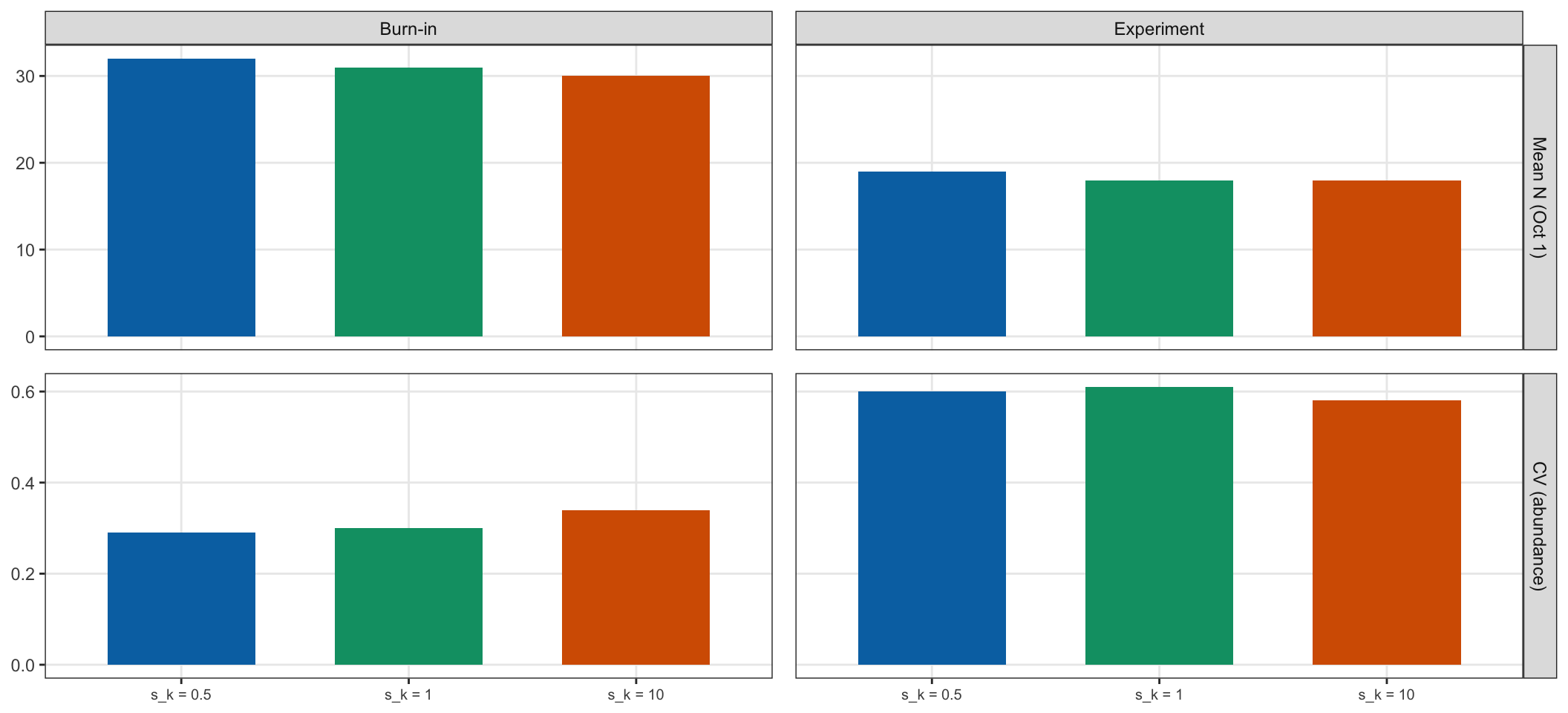
#| fig-cap: "Mean Oct 1 abundance and CV by s_k value, split by simulation phase."
#| fig-height: 5
plot_stability_fig(sk_stable, sk_cols)
```
```{r}
#| label: tbl-sk-stable
#| tbl-cap: "Stability statistics by s_k value."
sk_stable |>
  knitr::kable(col.names = c("s_k", "Phase", "Mean N",
                              "CV (abundance)", "Mean biomass (kg)", "Years"))
```
---
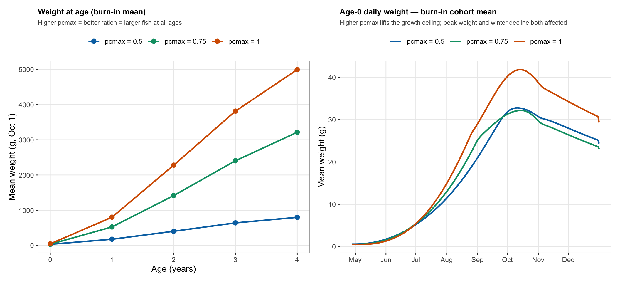
## `pcmax_cold` / `pcmax_warm`: maximum consumption
`pcmax` sets the ceiling on achievable daily consumption as a proportion of
physiological maximum Cmax. The effective ration is
`pcmax_adjusted = min(fT(temp), pcmax)`, so at peak summer cold-patch temperatures
(T ≈ 15°C, fT ≈ 0.91), `pcmax_cold = 0.5` is the binding constraint — fish are
food-limited by habitat quality, not by temperature. Raising pcmax relaxes this
ceiling and directly increases `pcmax_adjusted_dd` for all fish.
```{r}
#| label: sim-pcmax
#| cache: false
pcmax_vals   <- c(0.50, 0.75, 1.00)
pcmax_labels <- paste0("pcmax = ", pcmax_vals)
pcmax_cols   <- c("#0072B2", "#009E73", "#D55E00")

cache_file <- "cache/pcmax_sims.rds"
if (file.exists(cache_file)) {
  cat("Loading pcmax simulations from cache...\n")
  pcmax_sims <- readRDS(cache_file)
} else {
  cat("Running pcmax sensitivity simulations...\n")
  pcmax_sims <- lapply(seq_along(pcmax_vals), function(i) {
    pv <- pcmax_vals[i]
    cat(" pcmax =", pv, "... ")
    p   <- modifyList(baseline, list(pcmax_cold = pv, pcmax_warm = pv))
    hdf <- build_habitat(p)
    res <- run_simulation(hdf, p, wt_growth = wt.growth)
    cat("ends", format(max(res$ibm_long$date, na.rm = TRUE)), "\n")
    res
  })
  names(pcmax_sims) <- pcmax_labels
  dir.create("cache", showWarnings = FALSE)
  saveRDS(pcmax_sims, cache_file)
}
```
```{r}
#| label: pcmax-outcomes
pcmax_census   <- bind_rows(Map(oct1_census,   pcmax_sims, pcmax_labels)) |>
  mutate(label = factor(label, levels = pcmax_labels))
pcmax_sr       <- bind_rows(Map(stock_recruit, pcmax_sims, pcmax_labels)) |>
  mutate(label = factor(label, levels = pcmax_labels))
pcmax_thin     <- bind_rows(Map(thinning_rate,        pcmax_sims, pcmax_labels)) |>
  mutate(label = factor(label, levels = pcmax_labels))
pcmax_dg       <- bind_rows(Map(age0_density_growth, pcmax_sims, pcmax_labels)) |>
  mutate(label = factor(label, levels = pcmax_labels))
pcmax_waa      <- bind_rows(Map(wt_at_age,     pcmax_sims, pcmax_labels)) |>
  mutate(label = factor(label, levels = pcmax_labels))
pcmax_age0_dly <- bind_rows(Map(age0_daily_wt, pcmax_sims, pcmax_labels)) |>
  mutate(label = factor(label, levels = pcmax_labels))
pcmax_stable   <- stability_stats(pcmax_census)
```
### Abundance and biomass
```{r}
#| label: fig-pcmax-ts
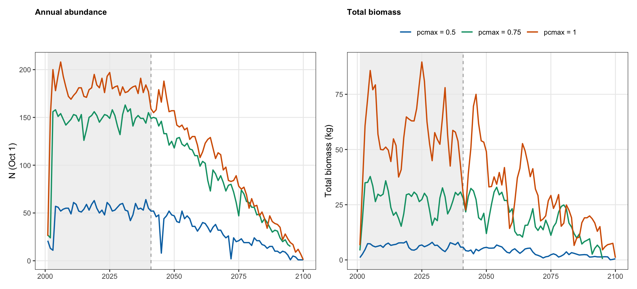
#| fig-cap: "Oct 1 abundance and biomass by pcmax value."
#| fig-height: 5
p_N <- ggplot(pcmax_census, aes(x = year, y = N, color = label)) +
  annotate("rect", xmin = burn_start, xmax = exp_start_yr,
           ymin = -Inf, ymax = Inf, fill = "grey92", alpha = 0.7) +
  geom_vline(xintercept = exp_start_yr, linetype = "dashed",
             color = "grey55", linewidth = 0.4) +
  geom_line(linewidth = 0.75) +
  scale_color_manual(values = pcmax_cols) +
  labs(x = NULL, y = "N (Oct 1)", color = NULL, title = "Annual abundance") +
  theme_sens() + theme(legend.position = "none")

p_B <- ggplot(pcmax_census, aes(x = year, y = biomass_kg, color = label)) +
  annotate("rect", xmin = burn_start, xmax = exp_start_yr,
           ymin = -Inf, ymax = Inf, fill = "grey92", alpha = 0.7) +
  geom_vline(xintercept = exp_start_yr, linetype = "dashed",
             color = "grey55", linewidth = 0.4) +
  geom_line(linewidth = 0.75) +
  scale_color_manual(values = pcmax_cols) +
  labs(x = NULL, y = "Total biomass (kg)", color = NULL, title = "Total biomass") +
  theme_sens()

p_N | p_B
```
### Compensatory dynamics
```{r}
#| label: fig-pcmax-comp
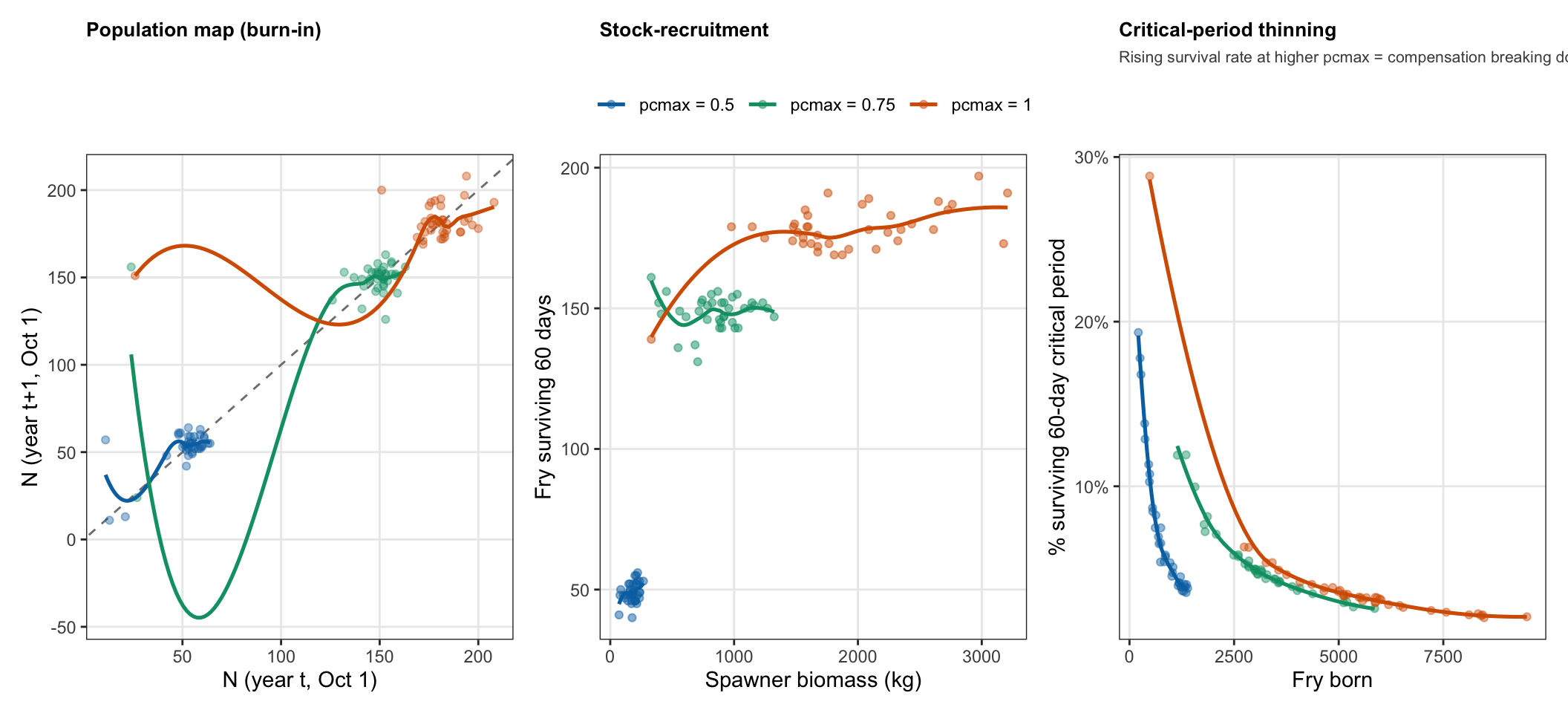
#| fig-cap: "Top-left: burn-in population map. Top-right: stock-recruitment. Bottom-left: size-based early thinning (% of fry surviving to day 60). Bottom-right: density–growth relationship. The bottom row together shows the two pathways of size-based density-dependent compensation: cohort thinning (left) and growth suppression (right). Weakening compensation at higher pcmax indicates threshold recalibration is needed."
#| fig-height: 8
pcmax_map <- pop_map(pcmax_census)

p_map <- ggplot(pcmax_map, aes(x = N, y = N_next, color = label)) +
  geom_abline(slope = 1, intercept = 0, linetype = "dashed", color = "grey50") +
  geom_point(alpha = 0.4, size = 1.5) +
  geom_smooth(method = "loess", se = FALSE, span = 0.75, linewidth = 0.9) +
  scale_color_manual(values = pcmax_cols) +
  labs(x = "N (year t, Oct 1)", y = "N (year t+1, Oct 1)", color = NULL,
       title = "Population map (burn-in)") +
  theme_sens() + theme(legend.position = "none")

p_sr <- ggplot(pcmax_sr |> filter(spawner_kg > 0),
               aes(x = spawner_kg, y = bio_surv60_kg, color = label)) +
  geom_point(alpha = 0.5, size = 1.5) +
  geom_smooth(method = "loess", se = FALSE, span = 0.7, linewidth = 0.9) +
  scale_color_manual(values = pcmax_cols) +
  labs(x = "Spawner biomass (kg)", y = "Fry biomass at 60 days (kg)", color = NULL,
       title = "Stock-recruitment") +
  theme_sens() + theme(legend.position = "right")

p_thin <- ggplot(pcmax_thin, aes(x = n_born, y = surv_rate, color = label)) +
  geom_point(alpha = 0.45, size = 1.5) +
  geom_smooth(method = "loess", se = FALSE, span = 0.7, linewidth = 0.9) +
  scale_y_continuous(labels = scales::percent_format(accuracy = 1)) +
  scale_color_manual(values = pcmax_cols) +
  labs(x = "Fry born", y = "% of fry surviving to day 60",
       color = NULL, title = "Size-based thinning",
       subtitle = "Rising survival rate at higher pcmax = compensation breaking down") +
  theme_sens() + theme(legend.position = "none")

p_dg <- ggplot(pcmax_dg, aes(x = mean_july_n, y = mean_wt, color = label)) +
  geom_point(alpha = 0.5, size = 1.5) +
  geom_smooth(method = "lm", se = FALSE, linewidth = 0.9) +
  geom_hline(yintercept = 7, linetype = "dotted", color = "grey50") +
  scale_color_manual(values = pcmax_cols) +
  labs(x = "Mean July N (all fish)", y = "Age-0 weight at Aug 1 (g)", color = NULL,
       title = "Density\u2013growth relationship",
       subtitle = "Higher density = slower early growth = more time below w\u2080") +
  theme_sens() + theme(legend.position = "none")

(p_map | p_sr) / (p_thin | p_dg)
```
### Age structure
```{r}
#| label: fig-pcmax-age0
#| fig-cap: "Left: mean weight at age (burn-in). Right: age-0 daily weight by day of year, averaged across burn-in cohorts."
#| fig-height: 5
p_waa <- ggplot(pcmax_waa, aes(x = age_yrs, y = mean_wt, color = label)) +
  geom_line(linewidth = 0.9) +
  geom_point(size = 2.5) +
  scale_color_manual(values = pcmax_cols) +
  scale_x_continuous(breaks = 0:4) +
  labs(x = "Age (years)", y = "Mean weight (g, Oct 1)",
       color = NULL, title = "Weight at age (burn-in mean)",
       subtitle = "Higher pcmax = better ration = larger fish at all ages") +
  theme_sens()

p_aget <- ggplot(pcmax_age0_dly |> filter(doy >= 118),
                 aes(x = doy, y = mean_wt, color = label)) +
  geom_line(linewidth = 0.9) +
  scale_color_manual(values = pcmax_cols) +
  scale_x_continuous(breaks = month_doys, labels = month_labels) +
  labs(x = NULL, y = "Mean weight (g)", color = NULL,
       title = "Age-0 daily weight — burn-in cohort mean",
       subtitle = "Higher pcmax lifts the growth ceiling; peak weight and winter decline both affected") +
  theme_sens()

p_waa | p_aget
```
### Density-dependent duration below s_w0
```{r}
#| label: fig-pcmax-danger-duration
#| fig-cap: "Days post-hatch until cohort-mean weight first exceeds s_w0, vs fry born. Each point is one burn-in cohort year; lines are OLS fits with 95% CI."
#| fig-height: 5
pcmax_cross <- bind_rows(Map(days_to_threshold, pcmax_sims, pcmax_labels)) |>
  mutate(label = factor(label, levels = pcmax_labels))

plot_danger_duration(pcmax_cross, pcmax_cols)
```
### Stability summary {.unnumbered}
```{r}
#| label: fig-pcmax-stable
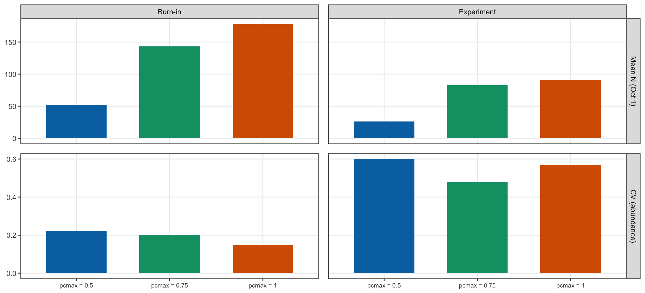
#| fig-cap: "Stability by pcmax."
#| fig-height: 5
plot_stability_fig(pcmax_stable, pcmax_cols)
```
```{r}
#| label: tbl-pcmax-stable
#| tbl-cap: "Stability statistics by pcmax."
pcmax_stable |>
  knitr::kable(col.names = c("pcmax", "Phase", "Mean N",
                              "CV (abundance)", "Mean biomass (kg)", "Years"))
```
---
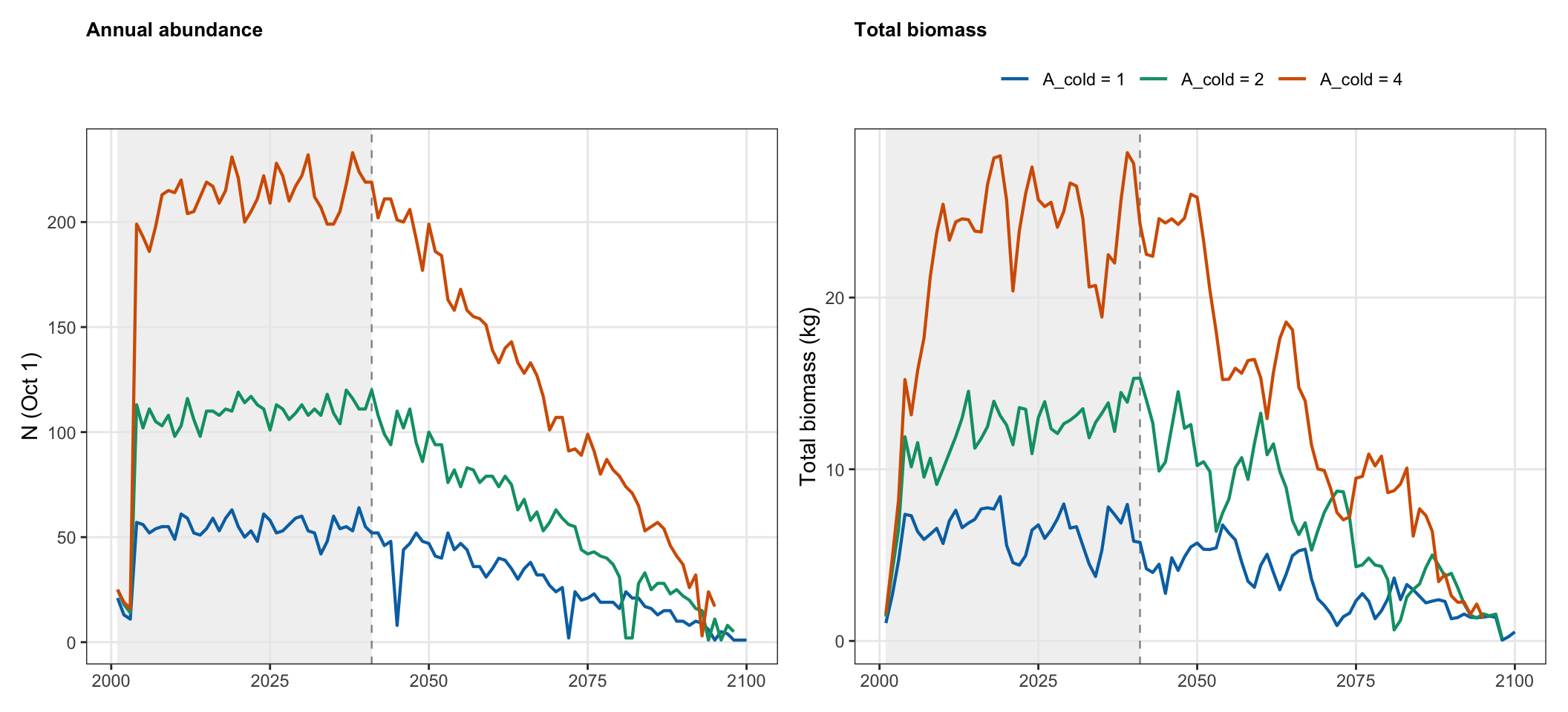
## `A_cold`: habitat area
`A_cold` sets the area of cold habitat available to fish (in arbitrary area units;
`eff_density = (n - 1) / A_cold`). For the null cold-only scenario, `A_warm = 0`
throughout, and cold habitat declines linearly from `A_cold` to 0 over the 60-year
experiment period regardless of starting area. Larger starting area means a larger
effective carrying capacity during the burn-in and a longer absolute decline before
the population is forced into critically small habitat.
::: {.callout-warning}
## Interaction with K
Increasing `A_cold` is mathematically equivalent to scaling K upward: both reduce
`eff_density` for a given N. **K and A_cold are partially substitutable**
:::
```{r}
#| label: sim-area
#| cache: false
area_vals   <- c(1, 2, 4)
area_labels <- paste0("A_cold = ", area_vals)
area_cols   <- c("#0072B2", "#009E73", "#D55E00")

cache_file <- "cache/area_sims.rds"
if (file.exists(cache_file)) {
  cat("Loading habitat area simulations from cache...\n")
  area_sims <- readRDS(cache_file)
} else {
  cat("Running habitat area sensitivity simulations...\n")
  area_sims <- lapply(seq_along(area_vals), function(i) {
    av <- area_vals[i]
    cat(" A_cold =", av, "... ")
    # A_cold_target = 0 retained: cold habitat still declines to 0 over experiment.
    # A_warm = 0 retained: null cold-only scenario.
    p   <- modifyList(baseline, list(A_cold = av))
    hdf <- build_habitat(p)
    res <- run_simulation(hdf, p, wt_growth = wt.growth)
    cat("ends", format(max(res$ibm_long$date, na.rm = TRUE)), "\n")
    res
  })
  names(area_sims) <- area_labels
  dir.create("cache", showWarnings = FALSE)
  saveRDS(area_sims, cache_file)
}
```
```{r}
#| label: area-outcomes
area_census   <- bind_rows(Map(oct1_census,   area_sims, area_labels)) |>
  mutate(label = factor(label, levels = area_labels))
area_sr       <- bind_rows(Map(stock_recruit, area_sims, area_labels)) |>
  mutate(label = factor(label, levels = area_labels))
area_thin     <- bind_rows(Map(thinning_rate,        area_sims, area_labels)) |>
  mutate(label = factor(label, levels = area_labels))
area_dg       <- bind_rows(Map(age0_density_growth, area_sims, area_labels)) |>
  mutate(label = factor(label, levels = area_labels))
area_waa      <- bind_rows(Map(wt_at_age,     area_sims, area_labels)) |>
  mutate(label = factor(label, levels = area_labels))
area_age0_dly <- bind_rows(Map(age0_daily_wt, area_sims, area_labels)) |>
  mutate(label = factor(label, levels = area_labels))
area_stable   <- stability_stats(area_census)
```
### Abundance and biomass
```{r}
#| label: fig-area-ts
#| fig-cap: "Oct 1 abundance and biomass by cold habitat area. All scenarios decline to extinction as A_cold → 0; larger starting area supports a larger population and may delay collapse."
#| fig-height: 5
p_N <- ggplot(area_census, aes(x = year, y = N, color = label)) +
  annotate("rect", xmin = burn_start, xmax = exp_start_yr,
           ymin = -Inf, ymax = Inf, fill = "grey92", alpha = 0.7) +
  geom_vline(xintercept = exp_start_yr, linetype = "dashed",
             color = "grey55", linewidth = 0.4) +
  geom_line(linewidth = 0.75) +
  scale_color_manual(values = area_cols) +
  labs(x = NULL, y = "N (Oct 1)", color = NULL, title = "Annual abundance") +
  theme_sens() + theme(legend.position = "none")

p_B <- ggplot(area_census, aes(x = year, y = biomass_kg, color = label)) +
  annotate("rect", xmin = burn_start, xmax = exp_start_yr,
           ymin = -Inf, ymax = Inf, fill = "grey92", alpha = 0.7) +
  geom_vline(xintercept = exp_start_yr, linetype = "dashed",
             color = "grey55", linewidth = 0.4) +
  geom_line(linewidth = 0.75) +
  scale_color_manual(values = area_cols) +
  labs(x = NULL, y = "Total biomass (kg)", color = NULL, title = "Total biomass") +
  theme_sens()

p_N | p_B
```
### Compensatory dynamics
```{r}
#| label: fig-area-comp
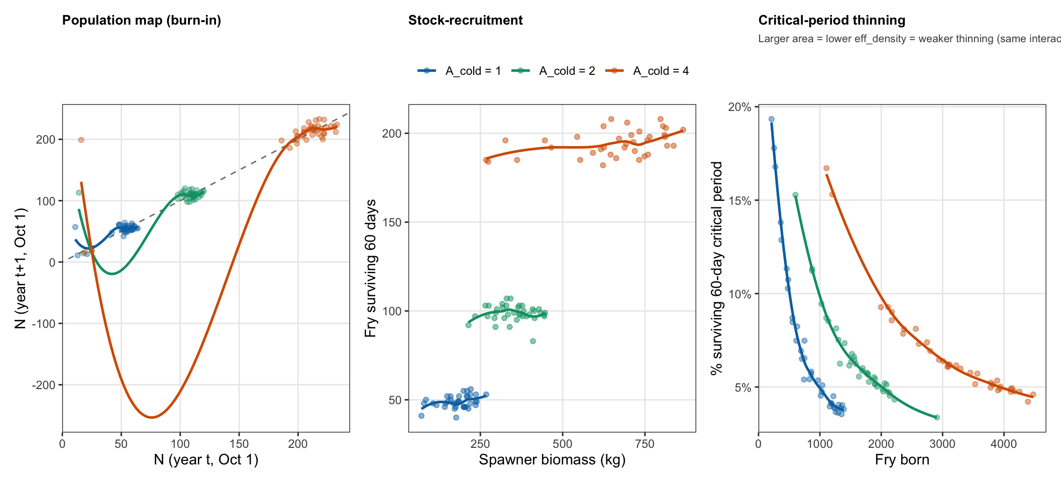
#| fig-cap: "Top-left: burn-in population map. Top-right: stock-recruitment. Bottom-left: size-based early thinning (% of fry surviving to day 60). Bottom-right: density–growth relationship. The bottom row together shows the two pathways of size-based density-dependent compensation: cohort thinning (left) and growth suppression (right)."
#| fig-height: 8
area_map <- pop_map(area_census)

p_map <- ggplot(area_map, aes(x = N, y = N_next, color = label)) +
  geom_abline(slope = 1, intercept = 0, linetype = "dashed", color = "grey50") +
  geom_point(alpha = 0.4, size = 1.5) +
  geom_smooth(method = "loess", se = FALSE, span = 0.75, linewidth = 0.9) +
  scale_color_manual(values = area_cols) +
  labs(x = "N (year t, Oct 1)", y = "N (year t+1, Oct 1)", color = NULL,
       title = "Population map (burn-in)") +
  theme_sens() + theme(legend.position = "none")

p_sr <- ggplot(area_sr |> filter(spawner_kg > 0),
               aes(x = spawner_kg, y = bio_surv60_kg, color = label)) +
  geom_point(alpha = 0.5, size = 1.5) +
  geom_smooth(method = "loess", se = FALSE, span = 0.7, linewidth = 0.9) +
  scale_color_manual(values = area_cols) +
  labs(x = "Spawner biomass (kg)", y = "Fry biomass at 60 days (kg)", color = NULL,
       title = "Stock-recruitment") +
  theme_sens() + theme(legend.position = "right")

p_thin <- ggplot(area_thin, aes(x = n_born, y = surv_rate, color = label)) +
  geom_point(alpha = 0.45, size = 1.5) +
  geom_smooth(method = "loess", se = FALSE, span = 0.7, linewidth = 0.9) +
  scale_y_continuous(labels = scales::percent_format(accuracy = 1)) +
  scale_color_manual(values = area_cols) +
  labs(x = "Fry born", y = "% of fry surviving to day 60",
       color = NULL, title = "Size-based thinning",
       subtitle = "Larger area = lower eff_density = weaker thinning (same interaction as high K)") +
  theme_sens() + theme(legend.position = "none")

p_dg <- ggplot(area_dg, aes(x = mean_july_n, y = mean_wt, color = label)) +
  geom_point(alpha = 0.5, size = 1.5) +
  geom_smooth(method = "lm", se = FALSE, linewidth = 0.9) +
  geom_hline(yintercept = 7, linetype = "dotted", color = "grey50") +
  scale_color_manual(values = area_cols) +
  labs(x = "Mean July N (all fish)", y = "Age-0 weight at Aug 1 (g)", color = NULL,
       title = "Density\u2013growth relationship",
       subtitle = "Higher density = slower early growth = more time below w\u2080") +
  theme_sens() + theme(legend.position = "none")

(p_map | p_sr) / (p_thin | p_dg)
```
### Age structure
```{r}
#| label: fig-area-age0
#| fig-cap: "Left: mean weight at age (burn-in). Right: age-0 daily weight by day of year, averaged across burn-in cohorts."
#| fig-height: 5
p_waa <- ggplot(area_waa, aes(x = age_yrs, y = mean_wt, color = label)) +
  geom_line(linewidth = 0.9) +
  geom_point(size = 2.5) +
  scale_color_manual(values = area_cols) +
  scale_x_continuous(breaks = 0:4) +
  labs(x = "Age (years)", y = "Mean weight (g, Oct 1)",
       color = NULL, title = "Weight at age (burn-in mean)",
       subtitle = "Larger area = lower competition = better individual growth") +
  theme_sens()

p_aget <- ggplot(area_age0_dly |> filter(doy >= 118),
                 aes(x = doy, y = mean_wt, color = label)) +
  geom_line(linewidth = 0.9) +
  scale_color_manual(values = area_cols) +
  scale_x_continuous(breaks = month_doys, labels = month_labels) +
  labs(x = NULL, y = "Mean weight (g)", color = NULL,
       title = "Age-0 daily weight — burn-in cohort mean") +
  theme_sens()

p_waa | p_aget
```
### Density-dependent duration below s_w0
```{r}
#| label: fig-area-danger-duration
#| fig-cap: "Days post-hatch until cohort-mean weight first exceeds s_w0, vs fry born. Each point is one burn-in cohort year; lines are OLS fits with 95% CI."
#| fig-height: 5
area_cross <- bind_rows(Map(days_to_threshold, area_sims, area_labels)) |>
  mutate(label = factor(label, levels = area_labels))

plot_danger_duration(area_cross, area_cols)
```
### Stability summary {.unnumbered}
```{r}
#| label: fig-area-stable
#| fig-cap: "Stability by cold habitat area."
#| fig-height: 5
plot_stability_fig(area_stable, area_cols)
```
```{r}
#| label: tbl-area-stable
#| tbl-cap: "Stability statistics by cold habitat area. Experiment years are comparable across scenarios only if populations survive long enough; earlier collapse at smaller area is expected."
area_stable |>
  knitr::kable(col.names = c("A_cold", "Phase", "Mean N",
                              "CV (abundance)", "Mean biomass (kg)", "Years"))
```
---
## Size and age structured competition (`age_structured_competition` × `dominance_beta`)
`age_structured_competition` controls whether fry (age-0) and older fish (age-1+)
compete as separate pools. When `TRUE`, fry compete only with other fry and adults
only with other adults, reflecting ontogenetic habitat segregation (channel margins
vs. pools and runs). When `FALSE`, all fish in a patch compete in one pool.
The effect of this toggle depends critically on `dominance_beta`:
- At **β = 1** adults are already near-immune to fry competition — a fry imposes a
competitive cost of `(m_fry / m_adult)^1 ≈ 0` on a large adult regardless of
age-class structuring. The toggle has little practical effect.
- At **β = 0.5** a fry imposes `(m_fry / m_adult)^0.5 ≈ 0.05` — non-trivial — so
adults feel meaningful fry competition when structuring is off.
This section uses a **2×2 design** (age_structured × dominance_beta) to make the
interaction explicit. `sim_crit` (TRUE, β = 1) and `sim_b05` (TRUE, β = 0.5) are
aliased from `beta_sims`; two new simulations complete the grid.
```{r}
#| label: sim-agestr
#| cache: false
# Pull the structured runs directly from beta_sims (baseline has
# age_structured_competition = TRUE, so these are identical to sim_crit / sim_b05)
sim_crit <- beta_sims[["β = 1"]]
sim_b05  <- beta_sims[["β = 0.5"]]

cache_file <- "cache/agestr_sims.rds"
if (file.exists(cache_file)) {
  cat("Loading age-structure simulations from cache...\n")
  agestr_cache     <- readRDS(cache_file)
  sim_agestr_F_b05 <- agestr_cache$sim_agestr_F_b05
  sim_agestr_F_b1  <- agestr_cache$sim_agestr_F_b1
} else {
  cat("Running age-class competition 2x2 simulations...\n")
  sim_agestr_F_b05 <- {
    cat(" age_structured=FALSE, beta=0.5 ... ")
    p   <- modifyList(baseline, list(age_structured_competition = FALSE,
                                     dominance_beta             = 0.5))
    res <- run_simulation(build_habitat(p), p, wt_growth = wt.growth)
    cat("ends", format(max(res$ibm_long$date, na.rm = TRUE)), "\n")
    res
  }
  sim_agestr_F_b1 <- {
    cat(" age_structured=FALSE, beta=1.0 ... ")
    p   <- modifyList(baseline, list(age_structured_competition = FALSE,
                                     dominance_beta             = 1))
    res <- run_simulation(build_habitat(p), p, wt_growth = wt.growth)
    cat("ends", format(max(res$ibm_long$date, na.rm = TRUE)), "\n")
    res
  }
  dir.create("cache", showWarnings = FALSE)
  saveRDS(list(sim_agestr_F_b05 = sim_agestr_F_b05,
               sim_agestr_F_b1  = sim_agestr_F_b1),
          cache_file)
}
```
```{r}
#| label: agestr-outcomes
agestr_sims <- list(
  "Structured, β = 1\n(baseline)" = sim_crit,
  "Structured, β = 0.5"           = sim_b05,
  "Unstructured, β = 1"           = sim_agestr_F_b1,
  "Unstructured, β = 0.5"         = sim_agestr_F_b05
)
agestr_labels <- names(agestr_sims)

# Colour = beta; linetype = competition structure
agestr_cols <- c("β = 1" = "#D55E00", "β = 0.5" = "#0072B2")
agestr_lty  <- c("Structured" = "solid", "Unstructured" = "dashed")

mk_agestr <- function(df)
  df |>
    mutate(beta_lab = if_else(grepl("0\\.5", label), "β = 0.5", "β = 1"),
           str_lab  = if_else(grepl("Unstr", label), "Unstructured", "Structured"))

agestr_census <- bind_rows(Map(oct1_census,   agestr_sims, agestr_labels)) |>
  mutate(label = factor(label, levels = agestr_labels)) |> mk_agestr()
agestr_thin   <- bind_rows(Map(thinning_rate, agestr_sims, agestr_labels)) |>
  mutate(label = factor(label, levels = agestr_labels)) |> mk_agestr()
agestr_waa    <- bind_rows(Map(wt_at_age,     agestr_sims, agestr_labels)) |>
  mutate(label = factor(label, levels = agestr_labels)) |> mk_agestr()
agestr_stable <- stability_stats(agestr_census)
```
### Abundance over time and population map
```{r}
#| label: fig-agestr-ts
#| fig-cap: "Oct 1 abundance and burn-in population map for the 2×2 age-structured × beta design. Colour = beta; linetype = competition structure."
#| fig-height: 9
p_ts <- ggplot(agestr_census,
               aes(x = year, y = N, color = beta_lab, linetype = str_lab)) +
  annotate("rect", xmin = burn_start, xmax = exp_start_yr,
           ymin = -Inf, ymax = Inf, fill = "grey92", alpha = 0.7) +
  geom_vline(xintercept = exp_start_yr, linetype = "dashed",
             color = "grey55", linewidth = 0.35) +
  geom_line(linewidth = 0.8) +
  scale_color_manual(values = agestr_cols) +
  scale_linetype_manual(values = agestr_lty) +
  labs(x = NULL, y = "N (Oct 1)", color = "dominance_beta",
       linetype = "Competition structure",
       title = "A: Annual abundance",
       subtitle = "Divergence between solid and dashed of same colour shows effect of age-class structuring") +
  theme_sens()

agestr_map <- agestr_census |>
  filter(phase == "burn-in") |>
  group_by(label, beta_lab, str_lab) |> arrange(year) |>
  mutate(N_next = lead(N)) |> ungroup() |> filter(!is.na(N_next))

p_map <- ggplot(agestr_map,
                aes(x = N, y = N_next, color = beta_lab, linetype = str_lab)) +
  geom_abline(slope = 1, intercept = 0, linetype = "dashed", color = "grey50") +
  geom_point(alpha = 0.4, size = 1.5) +
  geom_smooth(method = "loess", se = FALSE, span = 0.75, linewidth = 0.9) +
  scale_color_manual(values = agestr_cols) +
  scale_linetype_manual(values = agestr_lty) +
  labs(x = "N (year t, Oct 1)", y = "N (year t+1, Oct 1)",
       color = "dominance_beta", linetype = "Competition structure",
       title = "B: Population map (burn-in only)") +
  theme_sens()

p_ts / p_map
```
### Size-based thinning and weight at age
```{r}
#| label: fig-agestr-thin
#| fig-cap: "Thinning rate and weight-at-age for the 2×2 design."
#| fig-height: 5
p_thin <- ggplot(agestr_thin,
                 aes(x = n_born, y = surv_rate,
                     color = beta_lab, linetype = str_lab)) +
  geom_point(alpha = 0.4, size = 1.5) +
  geom_smooth(method = "loess", se = FALSE, span = 0.7, linewidth = 0.9) +
  scale_y_continuous(labels = scales::percent_format(accuracy = 1)) +
  scale_color_manual(values = agestr_cols) +
  scale_linetype_manual(values = agestr_lty) +
  labs(x = "Fry born", y = "% surviving 60 days",
       color = "dominance_beta", linetype = "Competition structure",
       title = "Size-based thinning") +
  theme_sens() + theme(legend.position = "none")

p_waa <- ggplot(agestr_waa,
                aes(x = age_yrs, y = mean_wt,
                    color = beta_lab, linetype = str_lab)) +
  geom_line(linewidth = 0.9) + geom_point(size = 2.5) +
  scale_color_manual(values = agestr_cols) +
  scale_linetype_manual(values = agestr_lty) +
  scale_x_continuous(breaks = 0:4) +
  labs(x = "Age (years)", y = "Mean weight (g, Oct 1)",
       color = "dominance_beta", linetype = "Competition structure",
       title = "Weight at age (burn-in mean)") +
  theme_sens()

p_thin | p_waa
```
### Stability summary {.unnumbered}
```{r}
#| label: tbl-agestr-stable
#| tbl-cap: "Stability statistics for the 2×2 age-class structured competition design."
agestr_stable |>
  knitr::kable(col.names = c("Scenario", "Phase", "Mean N",
                              "CV (abundance)", "Mean biomass (kg)", "Years"))
```
---
## Cross-parameter summary
```{r}
#| label: fig-cv-summary
#| fig-width: 13
#| fig-height: 13
#| fig-cap: "Sensitivity analysis summary. Row 1: mean Oct 1 abundance. Row 2: CV of abundance (lower = more stable). Row 3: total years simulated (burn-in + experiment; < 40 = collapsed before burn-in end). Row 4: peak mean age-0 weight (g) — the burn-in cohort-mean weight trajectory maximum, a summary of early growth potential under each parameter value. Row 5: among-cohort average time (days) to escape the critical period for survival (the size-based survival inflection weight, s_w0)."
param_levels <- c("K_cold", "egg_surv", "dominance_beta",
                  "pcmax_cold/warm", "A_cold",
                  "s_min", "s_w0", "s_k")
param_labels <- c("K", "egg_surv", "dom.\nbeta",
                  "pcmax\ncold/warm", "A_cold",
                  "s_min", "s_w0", "s_k")

# Mean length in days of the critical period (time to escape the period of reduced juvenile survival) per label
critical_time_all <- bind_rows(
  K_cross     |> group_by(label) |> summarise(critical_time = mean(days_to_cross, na.rm = TRUE), .groups = "drop") |> mutate(parameter = "K_cold"),
  egg_cross   |> group_by(label) |> summarise(critical_time = mean(days_to_cross, na.rm = TRUE), .groups = "drop") |> mutate(parameter = "egg_surv"),
  beta_cross  |> group_by(label) |> summarise(critical_time = mean(days_to_cross, na.rm = TRUE), .groups = "drop") |> mutate(parameter = "dominance_beta"),
  pcmax_cross |> group_by(label) |> summarise(critical_time = mean(days_to_cross, na.rm = TRUE), .groups = "drop") |> mutate(parameter = "pcmax_cold/warm"),
  area_cross  |> group_by(label) |> summarise(critical_time = mean(days_to_cross, na.rm = TRUE), .groups = "drop") |> mutate(parameter = "A_cold"),
  s_min_cross |> group_by(label) |> summarise(critical_time = mean(days_to_cross, na.rm = TRUE), .groups = "drop") |> mutate(parameter = "s_min"),
  w0_cross    |> group_by(label) |> summarise(critical_time = mean(days_to_cross, na.rm = TRUE), .groups = "drop") |> mutate(parameter = "s_w0"),
  sk_cross    |> group_by(label) |> summarise(critical_time = mean(days_to_cross, na.rm = TRUE), .groups = "drop") |> mutate(parameter = "s_k")
)

# Peak age-0 daily weight (max of burn-in cohort-mean trajectory) per label
peak_age0_all <- bind_rows(
  K_age0_dly     |> group_by(label) |> summarise(peak_age0_wt = max(mean_wt, na.rm = TRUE), .groups = "drop") |> mutate(parameter = "K_cold"),
  egg_age0_dly   |> group_by(label) |> summarise(peak_age0_wt = max(mean_wt, na.rm = TRUE), .groups = "drop") |> mutate(parameter = "egg_surv"),
  beta_age0_dly  |> group_by(label) |> summarise(peak_age0_wt = max(mean_wt, na.rm = TRUE), .groups = "drop") |> mutate(parameter = "dominance_beta"),
  pcmax_age0_dly |> group_by(label) |> summarise(peak_age0_wt = max(mean_wt, na.rm = TRUE), .groups = "drop") |> mutate(parameter = "pcmax_cold/warm"),
  area_age0_dly  |> group_by(label) |> summarise(peak_age0_wt = max(mean_wt, na.rm = TRUE), .groups = "drop") |> mutate(parameter = "A_cold"),
  s_min_age0_dly |> group_by(label) |> summarise(peak_age0_wt = max(mean_wt, na.rm = TRUE), .groups = "drop") |> mutate(parameter = "s_min"),
  w0_age0_dly    |> group_by(label) |> summarise(peak_age0_wt = max(mean_wt, na.rm = TRUE), .groups = "drop") |> mutate(parameter = "s_w0"),
  sk_age0_dly    |> group_by(label) |> summarise(peak_age0_wt = max(mean_wt, na.rm = TRUE), .groups = "drop") |> mutate(parameter = "s_k")
)

# Burn-in stability (mean N, CV) joined with total years across both phases
total_yrs_all <- bind_rows(
  total_sim_yrs(K_census)      |> mutate(parameter = "K_cold"),
  total_sim_yrs(egg_census)    |> mutate(parameter = "egg_surv"),
  total_sim_yrs(beta_census)   |> mutate(parameter = "dominance_beta"),
  total_sim_yrs(pcmax_census)  |> mutate(parameter = "pcmax_cold/warm"),
  total_sim_yrs(area_census)   |> mutate(parameter = "A_cold"),
  total_sim_yrs(s_min_census)  |> mutate(parameter = "s_min"),
  total_sim_yrs(w0_census)     |> mutate(parameter = "s_w0"),
  total_sim_yrs(sk_census)     |> mutate(parameter = "s_k")
)

cv_all <- bind_rows(
  K_stable      |> filter(phase == "burn-in") |> mutate(parameter = "K_cold"),
  egg_stable    |> filter(phase == "burn-in") |> mutate(parameter = "egg_surv"),
  beta_stable   |> filter(phase == "burn-in") |> mutate(parameter = "dominance_beta"),
  pcmax_stable  |> filter(phase == "burn-in") |> mutate(parameter = "pcmax_cold/warm"),
  area_stable   |> filter(phase == "burn-in") |> mutate(parameter = "A_cold"),
  s_min_stable  |> filter(phase == "burn-in") |> mutate(parameter = "s_min"),
  w0_stable     |> filter(phase == "burn-in") |> mutate(parameter = "s_w0"),
  sk_stable     |> filter(phase == "burn-in") |> mutate(parameter = "s_k")
) |>
  left_join(total_yrs_all,  by = c("label", "parameter")) |>
  left_join(peak_age0_all, by = c("label", "parameter")) |>
  left_join(critical_time_all, by = c("label", "parameter")) |>
  mutate(parameter = factor(parameter, levels = param_levels,
                            labels = param_labels))

cv_all_long <- cv_all |>
  pivot_longer(c(mean_N, cv, total_yrs, peak_age0_wt, critical_time),
               names_to  = "metric",
               values_to = "value") |>
  mutate(metric = factor(metric,
                         levels = c("mean_N", "cv", "total_yrs", "peak_age0_wt", "critical_time"),
                         labels = c("Mean N (Oct 1)",
                                    "CV (abundance)",
                                    "Years simulated (max = 100)",
                                    "Peak age-0 weight (g)",
                                    "Critical period (days)")))

# Okabe-Ito 8-color palette (colorblind-friendly)
param_fill <- c("#0072B2", "#009E73", "#D55E00", "#56B4E9", "#999999",
                "#E69F00", "#CC79A7", "#000000")
names(param_fill) <- param_labels

ggplot(cv_all_long, aes(x = label, y = value, fill = parameter)) +
  geom_col(width = 0.65, show.legend = FALSE) +
  # Year 40: end of burn-in (bars below = collapsed during burn-in)
  geom_hline(
    data = \(d) filter(d, metric == "Years simulated (max = 100)"),
    aes(yintercept = 40),
    linetype = "dotted", color = "grey35", linewidth = 0.6
  ) +
  # Year 100: end of full simulation (bars below = collapsed during experiment)
  geom_hline(
    data = \(d) filter(d, metric == "Years simulated (max = 100)"),
    aes(yintercept = 100),
    linetype = "dashed", color = "grey35", linewidth = 0.6
  ) +
  facet_grid(metric ~ parameter, scales = "free") +
  scale_fill_manual(values = param_fill) +
  scale_y_continuous(expand = expansion(mult = c(0, 0.12))) +
  labs(x = NULL, y = NULL,
       title = "Burn-in stability across all parameter sensitivity analyses",
       subtitle = paste0(
         "Row 1: burn-in mean N.  Row 2: burn-in CV (lower = more stable).  ",
         "Row 3: total years simulated (burn-in + experiment). ",
         "Row 4: peak mean age-0 weight (g) — summarises early growth potential.  ",
         "Dotted = yr 40 (burn-in end); dashed = yr 100 (full simulation). "
         )) +
  theme_bw() +
  theme(strip.background  = element_rect(fill = "grey88"),
        strip.text.x      = element_text(size = 8),
        strip.text.y      = element_text(size = 7.5, lineheight = 0.85),
        panel.grid.minor  = element_blank(),
        axis.text.x       = element_text(size = 6.5, lineheight = 0.8),
        plot.title        = element_text(size = 10, face = "bold"),
        plot.subtitle     = element_text(size = 7.5, color = "grey30"),
        panel.spacing     = unit(0.6, "lines"))
```
### Age-class structured competition — 2×2 stability {.unnumbered}
The age-class section uses a factorial design rather than a single-axis sweep, so
it is not directly comparable to the single-parameter bar charts above. The table
below summarises burn-in stability for all four combinations.
```{r}
#| label: tbl-agestr-summary
#| tbl-cap: "Burn-in stability for the 2×2 age-structured × dominance_beta design. Rows where years simulated < 100 indicate premature collapse."
agestr_stable |>
  left_join(
    bind_rows(Map(function(s, l)
      tibble(label = l, total_yrs = n_distinct(
        year(s$ibm_long$date[!is.na(s$ibm_long$date)]))),
      agestr_sims, agestr_labels)),
    by = "label"
  ) |>
  filter(phase == "burn-in") |>
  select(label, mean_N, cv, total_yrs) |>
  knitr::kable(col.names = c("Scenario", "Burn-in mean N",
                              "Burn-in CV", "Total years simulated"))
```
## Final tune
This section runs a single candidate parameterisation that combines adjustments
identified during the sensitivity analysis: `egg_surv = 0.2` (higher egg-to-fry
survival than the baseline of 0.1), `s_w0 = 5` (a lower size-based survival
inflection weight), `s_k = 0.8` (a slightly lower inflection steepness), and
`K_cold/K_warm = 400` (a high half-saturation density, i.e., lower strength of
density density dependence). All other parameters are held at their baseline values.
The purpose is to assess whether this combination produces acceptable burn-in dynamics
and compensatory regulation before committing to it as the working parameterisation
for scenario runs.
```{r}
#| label: sim-final
#| cache: true
cat("Running final tune simulation...\n")
p          <- modifyList(baseline, list(egg_surv = 0.15, s_w0 = 5, s_k = 0.8, K_cold = 400, K_warm = 400))
hdf        <- build_habitat(p)
final_sims <- run_simulation(hdf, p, wt_growth = wt.growth)
cat("ends", format(max(final_sims$ibm_long$date, na.rm = TRUE)), "\n")
```
```{r}
#| label: final-outcomes
final_label   <- "egg_surv=0.15 / s_w0=5 / s_k=0.8 / K=400"
final_col     <- c("egg_surv=0.15 / s_w0=5 / s_k=0.8 / K=400" = "#009E73")

final_census  <- oct1_census(         final_sims, final_label)
final_sr      <- stock_recruit(        final_sims, final_label)
final_thin    <- thinning_rate(        final_sims, final_label)
final_dg      <- age0_density_growth(  final_sims, final_label)
final_waa     <- wt_at_age(            final_sims, final_label)
final_age0_dly <- age0_daily_wt(       final_sims, final_label)
final_stable  <- stability_stats(final_census)
final_cross   <- days_to_threshold(    final_sims, final_label)
```
### Abundance and biomass
```{r}
#| label: fig-final-ts
#| fig-cap: "Oct 1 annual abundance and total biomass for the final-tune parameterisation. Grey band = burn-in."
#| fig-height: 5
p_N <- ggplot(final_census, aes(x = year, y = N)) +
  annotate("rect", xmin = burn_start, xmax = exp_start_yr,
           ymin = -Inf, ymax = Inf, fill = "grey92", alpha = 0.7) +
  geom_vline(xintercept = exp_start_yr, linetype = "dashed",
             color = "grey55", linewidth = 0.4) +
  geom_line(linewidth = 0.75, color = "#009E73") +
  labs(x = NULL, y = "N (Oct 1)", title = "Annual abundance") +
  theme_sens()

p_B <- ggplot(final_census, aes(x = year, y = biomass_kg)) +
  annotate("rect", xmin = burn_start, xmax = exp_start_yr,
           ymin = -Inf, ymax = Inf, fill = "grey92", alpha = 0.7) +
  geom_vline(xintercept = exp_start_yr, linetype = "dashed",
             color = "grey55", linewidth = 0.4) +
  geom_line(linewidth = 0.75, color = "#009E73") +
  labs(x = NULL, y = "Total biomass (kg)", title = "Total biomass") +
  theme_sens()

p_N | p_B
```
### Compensatory dynamics
```{r}
#| label: fig-final-comp
#| fig-cap: "Top-left: burn-in population map. Top-right: stock-recruitment. Bottom-left: size-based early thinning (% of fry surviving to day 60). Bottom-right: density–growth relationship. The bottom row together shows the two pathways of size-based density-dependent compensation: cohort thinning (left) and growth suppression (right)."
#| fig-height: 8
final_map <- pop_map(final_census)

p_map <- ggplot(final_map, aes(x = N, y = N_next)) +
  geom_abline(slope = 1, intercept = 0, linetype = "dashed", color = "grey50") +
  geom_point(alpha = 0.4, size = 1.5, color = "#009E73") +
  geom_smooth(method = "loess", se = FALSE, span = 0.75,
              linewidth = 0.9, color = "#009E73") +
  labs(x = "N (year t, Oct 1)", y = "N (year t+1, Oct 1)",
       title = "Population map (burn-in)") +
  theme_sens()

p_sr <- ggplot(final_sr |> filter(spawner_kg > 0),
               aes(x = spawner_kg, y = bio_surv60_kg)) +
  geom_point(alpha = 0.5, size = 1.5, color = "#009E73") +
  geom_smooth(method = "loess", se = FALSE, span = 0.7,
              linewidth = 0.9, color = "#009E73") +
  labs(x = "Spawner biomass (kg)", y = "Fry biomass at 60 days (kg)",
       title = "Stock-recruitment") +
  theme_sens()

p_thin <- ggplot(final_thin, aes(x = n_born, y = surv_rate)) +
  geom_point(alpha = 0.45, size = 1.5, color = "#009E73") +
  geom_smooth(method = "loess", se = FALSE, span = 0.7,
              linewidth = 0.9, color = "#009E73") +
  scale_y_continuous(labels = scales::percent_format(accuracy = 1)) +
  labs(x = "Fry born", y = "% of fry surviving to day 60",
       title = "Size-based thinning") +
  theme_sens()

p_dg <- ggplot(final_dg, aes(x = mean_july_n, y = mean_wt)) +
  geom_point(alpha = 0.5, size = 1.5, color = "#009E73") +
  geom_smooth(method = "lm", se = FALSE, linewidth = 0.9, color = "#009E73") +
  geom_hline(yintercept = 7, linetype = "dotted", color = "grey50") +
  labs(x = "Mean July N (all fish)", y = "Age-0 weight at Aug 1 (g)",
       title = "Density\u2013growth relationship",
       subtitle = "Higher density = slower early growth = more time below w\u2080") +
  theme_sens()

(p_map | p_sr) / (p_thin | p_dg)
```
### Age structure
```{r}
#| label: fig-final-age0
#| fig-cap: "Left: mean weight at age (burn-in). Right: age-0 daily weight by day of year, averaged across burn-in cohorts."
#| fig-height: 5
p_waa <- ggplot(final_waa, aes(x = age_yrs, y = mean_wt)) +
  geom_line(linewidth = 0.9, color = "#009E73") +
  geom_point(size = 2.5, color = "#009E73") +
  scale_x_continuous(breaks = 0:4) +
  labs(x = "Age (years)", y = "Mean weight (g, Oct 1)",
       title = "Weight at age (burn-in mean)") +
  theme_sens()

p_aget <- ggplot(final_age0_dly |> filter(doy >= 118),
                 aes(x = doy, y = mean_wt)) +
  geom_line(linewidth = 0.9, color = "#009E73") +
  scale_x_continuous(breaks = month_doys, labels = month_labels) +
  labs(x = NULL, y = "Mean weight (g)",
       title = "Age-0 daily weight \u2014 burn-in cohort mean") +
  theme_sens()

p_waa | p_aget
```
### Density-dependent duration below s_w0
```{r}
#| label: fig-final-danger-duration
#| fig-cap: "Days post-hatch until cohort-mean weight first exceeds s_w0, vs fry born. Each point is one burn-in cohort year; line is an OLS fit with 95% CI."
#| fig-height: 5
plot_danger_duration(final_cross, final_col)
```
### Stability summary {.unnumbered}
```{r}
#| label: fig-final-stable
#| fig-cap: "Mean Oct 1 abundance and CV for the final-tune parameterisation, split by simulation phase."
#| fig-height: 5
plot_stability_fig(final_stable, final_col)
```
```{r}
#| label: tbl-final-stable
#| tbl-cap: "Stability statistics for the final-tune parameterisation."
final_stable |>
  knitr::kable(col.names = c("Scenario", "Phase", "Mean N",
                              "CV (abundance)", "Mean biomass (kg)", "Years"))
```