---
title: "Surplus Production"
---
```{r, include = FALSE, cache = FALSE}
library(tidyverse)
library(lubridate)
library(ggpubr)
library(egg)
library(RColorBrewer)
library(ggridges)
library(patchwork)
library(scales)
library(ggrepel)
source("Functions.R")
source("PlotResults.R")
source("ScenarioDefs.R")
```
**Purpose:** Compare surplus production and the impacts of "harvest" across habitat scenarios.
## Setup
Load relevant .rds objects and bind directly into a list. Using a helper function ensures each `res` object is freed from memory as soon as `ibm_long` is extracted, avoiding duplicate references that would force R to copy the data frames.
```{r}
#| cache: false
# get experiment start date from base parameters
exp_start_date <- base_params$mindate + years(base_params$nyears_burnin)

# Helper: read one scenario, extract ibm_long summaries, and free res before returning.
# Rather than storing the full ibm_long data frame (very large), we pre-extract the
# three filtered/aggregated subsets that are actually used downstream:
#   oct1_exp   – Oct 1 weight-at-age rows for the experimental period
#   age0_nov1  – annual age-0 counts and biomass on Nov 1 (used in both the
#                Recruitment and Stock-Recruitment sections)
#   fry_annual – annual fry birth counts for the experimental period
load_scen <- function(path, ht, pc, ac, aw, hr, pcmax_cold, pcmax_warm) {
  res <- readRDS(path)
  ibm <- res$ibm_long

  oct1_exp <- ibm |>
    filter(date >= exp_start_date,
           month(date) == 10, day(date) == 1,
           survived == 1) |>
    mutate(yr = year(date), age_class = floor(age)) |>
    select(yr, age_class, weight, condition) %>%
    mutate(peak_weight = weight / condition)

  age0_nov1 <- ibm |>
    filter(date >= exp_start_date,
           month(date) == 11, day(date) == 1,
           survived == 1, floor(age) == 0) |>
    group_by(yr = year(date)) |>
    summarise(n_age0 = n(), biom_age0 = sum(weight), .groups = "drop")

  fry_annual <- ibm |>
    filter(date >= exp_start_date,
           !is.na(parent_pid),
           dayofsim == birth_dayofsim) |>
    count(yr = year(date), name = "n_fry")

  list(oct1_exp = oct1_exp, age0_nov1 = age0_nov1, fry_annual = fry_annual,
       harvest = res$harvest_log, spawn_log = res$spawn_log,
       ht = ht, pc = pc, ac = ac, aw = aw, hr = hr,
       pcmax_cold = pcmax_cold, pcmax_warm = pcmax_warm)
}

ibm_list_mech <- list(
  # PrCold = 50%
  load_scen("results/TempOffset_ColdOnly_50percold.rds",  "Cold only",  0.50,  1.0,  0.0,  0.00,  0.5,  NA_real_),
  load_scen("results/Harvest_10_ColdOnly_50percold.rds",  "Cold only",  0.50,  1.0,  0.0,  0.10,  0.5,  NA_real_),
  load_scen("results/Harvest_20_ColdOnly_50percold.rds",  "Cold only",  0.50,  1.0,  0.0,  0.20,  0.5,  NA_real_),
  load_scen("results/Harvest_30_ColdOnly_50percold.rds",  "Cold only",  0.50,  1.0,  0.0,  0.30,  0.5,  NA_real_),
  load_scen("results/Harvest_40_ColdOnly_50percold.rds",  "Cold only",  0.50,  1.0,  0.0,  0.40,  0.5,  NA_real_),
  load_scen("results/Harvest_50_ColdOnly_50percold.rds",  "Cold only",  0.50,  1.0,  0.0,  0.50,  0.5,  NA_real_),
  load_scen("results/Harvest_55_ColdOnly_50percold.rds",  "Cold only",  0.50,  1.0,  0.0,  0.55,  0.5,  NA_real_),
  load_scen("results/Harvest_60_ColdOnly_50percold.rds",  "Cold only",  0.50,  1.0,  0.0,  0.60,  0.5,  NA_real_),
  load_scen("results/Harvest_65_ColdOnly_50percold.rds",  "Cold only",  0.50,  1.0,  0.0,  0.65,  0.5,  NA_real_),
  load_scen("results/Harvest_70_ColdOnly_50percold.rds",  "Cold only",  0.50,  1.0,  0.0,  0.70,  0.5,  NA_real_),
  load_scen("results/Harvest_75_ColdOnly_50percold.rds",  "Cold only",  0.50,  1.0,  0.0,  0.75,  0.5,  NA_real_),
  load_scen("results/Harvest_80_ColdOnly_50percold.rds",  "Cold only",  0.50,  1.0,  0.0,  0.80,  0.5,  NA_real_),
  load_scen("results/Harvest_90_ColdOnly_50percold.rds",  "Cold only",  0.50,  1.0,  0.0,  0.90,  0.5,  NA_real_),

  load_scen("results/TempOffset_ColdWarm_50percold.rds",  "Cold + Warm",  0.50,  1.0,  1.0,  0.00,  0.5,  0.5),
  load_scen("results/Harvest_10_ColdWarm_50percold.rds",  "Cold + Warm",  0.50,  1.0,  1.0,  0.10,  0.5,  0.5),
  load_scen("results/Harvest_20_ColdWarm_50percold.rds",  "Cold + Warm",  0.50,  1.0,  1.0,  0.20,  0.5,  0.5),
  load_scen("results/Harvest_30_ColdWarm_50percold.rds",  "Cold + Warm",  0.50,  1.0,  1.0,  0.30,  0.5,  0.5),
  load_scen("results/Harvest_40_ColdWarm_50percold.rds",  "Cold + Warm",  0.50,  1.0,  1.0,  0.40,  0.5,  0.5),
  load_scen("results/Harvest_50_ColdWarm_50percold.rds",  "Cold + Warm",  0.50,  1.0,  1.0,  0.50,  0.5,  0.5),
  load_scen("results/Harvest_55_ColdWarm_50percold.rds",  "Cold + Warm",  0.50,  1.0,  1.0,  0.55,  0.5,  0.5),
  load_scen("results/Harvest_60_ColdWarm_50percold.rds",  "Cold + Warm",  0.50,  1.0,  1.0,  0.60,  0.5,  0.5),
  load_scen("results/Harvest_65_ColdWarm_50percold.rds",  "Cold + Warm",  0.50,  1.0,  1.0,  0.65,  0.5,  0.5),
  load_scen("results/Harvest_70_ColdWarm_50percold.rds",  "Cold + Warm",  0.50,  1.0,  1.0,  0.70,  0.5,  0.5),
  load_scen("results/Harvest_75_ColdWarm_50percold.rds",  "Cold + Warm",  0.50,  1.0,  1.0,  0.75,  0.5,  0.5),
  load_scen("results/Harvest_80_ColdWarm_50percold.rds",  "Cold + Warm",  0.50,  1.0,  1.0,  0.80,  0.5,  0.5),
  load_scen("results/Harvest_90_ColdWarm_50percold.rds",  "Cold + Warm",  0.50,  1.0,  1.0,  0.90,  0.5,  0.5),

  # PrCold = 25%
  load_scen("results/TempOffset_ColdOnly_25percold.rds",  "Cold only",  0.25,  0.5,  0.0,  0.00,  0.5,  NA_real_),
  load_scen("results/Harvest_10_ColdOnly_25percold.rds",  "Cold only",  0.25,  0.5,  0.0,  0.10,  0.5,  NA_real_),
  load_scen("results/Harvest_20_ColdOnly_25percold.rds",  "Cold only",  0.25,  0.5,  0.0,  0.20,  0.5,  NA_real_),
  load_scen("results/Harvest_30_ColdOnly_25percold.rds",  "Cold only",  0.25,  0.5,  0.0,  0.30,  0.5,  NA_real_),
  load_scen("results/Harvest_40_ColdOnly_25percold.rds",  "Cold only",  0.25,  0.5,  0.0,  0.40,  0.5,  NA_real_),
  load_scen("results/Harvest_50_ColdOnly_25percold.rds",  "Cold only",  0.25,  0.5,  0.0,  0.50,  0.5,  NA_real_),
  load_scen("results/Harvest_55_ColdOnly_25percold.rds",  "Cold only",  0.25,  0.5,  0.0,  0.55,  0.5,  NA_real_),
  load_scen("results/Harvest_60_ColdOnly_25percold.rds",  "Cold only",  0.25,  0.5,  0.0,  0.60,  0.5,  NA_real_),
  load_scen("results/Harvest_65_ColdOnly_25percold.rds",  "Cold only",  0.25,  0.5,  0.0,  0.65,  0.5,  NA_real_),
  load_scen("results/Harvest_70_ColdOnly_25percold.rds",  "Cold only",  0.25,  0.5,  0.0,  0.70,  0.5,  NA_real_),
  load_scen("results/Harvest_75_ColdOnly_25percold.rds",  "Cold only",  0.25,  0.5,  0.0,  0.75,  0.5,  NA_real_),
  load_scen("results/Harvest_80_ColdOnly_25percold.rds",  "Cold only",  0.25,  0.5,  0.0,  0.80,  0.5,  NA_real_),
  load_scen("results/Harvest_90_ColdOnly_25percold.rds",  "Cold only",  0.25,  0.5,  0.0,  0.90,  0.5,  NA_real_),

  load_scen("results/TempOffset_ColdWarm_25percold.rds",  "Cold + Warm",  0.25,  0.5,  1.5,  0.00,  0.5,  0.5),
  load_scen("results/Harvest_10_ColdWarm_25percold.rds",  "Cold + Warm",  0.25,  0.5,  1.5,  0.10,  0.5,  0.5),
  load_scen("results/Harvest_20_ColdWarm_25percold.rds",  "Cold + Warm",  0.25,  0.5,  1.5,  0.20,  0.5,  0.5),
  load_scen("results/Harvest_30_ColdWarm_25percold.rds",  "Cold + Warm",  0.25,  0.5,  1.5,  0.30,  0.5,  0.5),
  load_scen("results/Harvest_40_ColdWarm_25percold.rds",  "Cold + Warm",  0.25,  0.5,  1.5,  0.40,  0.5,  0.5),
  load_scen("results/Harvest_50_ColdWarm_25percold.rds",  "Cold + Warm",  0.25,  0.5,  1.5,  0.50,  0.5,  0.5),
  load_scen("results/Harvest_55_ColdWarm_25percold.rds",  "Cold + Warm",  0.25,  0.5,  1.5,  0.55,  0.5,  0.5),
  load_scen("results/Harvest_60_ColdWarm_25percold.rds",  "Cold + Warm",  0.25,  0.5,  1.5,  0.60,  0.5,  0.5),
  load_scen("results/Harvest_65_ColdWarm_25percold.rds",  "Cold + Warm",  0.25,  0.5,  1.5,  0.65,  0.5,  0.5),
  load_scen("results/Harvest_70_ColdWarm_25percold.rds",  "Cold + Warm",  0.25,  0.5,  1.5,  0.70,  0.5,  0.5),
  load_scen("results/Harvest_75_ColdWarm_25percold.rds",  "Cold + Warm",  0.25,  0.5,  1.5,  0.75,  0.5,  0.5),
  load_scen("results/Harvest_80_ColdWarm_25percold.rds",  "Cold + Warm",  0.25,  0.5,  1.5,  0.80,  0.5,  0.5),
  load_scen("results/Harvest_90_ColdWarm_25percold.rds",  "Cold + Warm",  0.25,  0.5,  1.5,  0.90,  0.5,  0.5)
)
```
Define misc. objects:
```{r}
#| cache: false
# ── Scenario metadata ─────────────────────────────────────────────────────────
scen_meta <- tibble(
  scen_key  = c("95", "75", "50", "25", "05"),
  label     = c("95% cold", "75% cold", "50% cold", "25% cold", "5% cold"),
  prop_cold = c(0.95, 0.75, 0.50, 0.25, 0.05)
)

# factor levels
pc_levels <- c(0.95, 0.75, 0.50, 0.25, 0.05)
pc_levels_mech <- c(0.95, 0.75, 0.50, 0.25, 0.05)
pc_labels_mech <- c("95% cold","75% cold","50% cold","25% cold","5% cold")

hr_levels <- c(0.00, 0.10, 0.20, 0.30, 0.40, 0.50, 0.55, 0.60, 0.65, 0.70, 0.75, 0.80, 0.9)
hr_levels_mech <- c(0.00, 0.10, 0.20, 0.30, 0.40, 0.50, 0.55, 0.60, 0.65, 0.70, 0.75, 0.80, 0.9)
hr_labels_mech <- c("0%","10%","20%","30%","40%", "50%", "55%", "60%", "65%", "70%", "75%", "80%", "90%")

# Palette keys must match levels(age0_ts$harvest_rate)
cols <- hcl.colors(13, "inferno", rev = TRUE)
hr_pal <- c("0%"  = "grey70", "10%" = cols[2], "20%" = cols[3], "30%" = cols[4],
            "40%" = cols[5], "50%" = cols[6], "55%" = cols[7], "60%" = cols[8],
            "65%" = cols[9], "70%" = cols[10], "75%" = cols[11], "80%" = cols[12],
            "90%" = cols[13])

# color palette for prop_cold
# scen_pal <- setNames(
#   hcl.colors(5, "Zissou 1"),
#   scen_meta$label
# )

# Linetype and shape palettes for habitat availability
hab_cols  <- c("Cold only" = "#6BAED6",  "Cold + Warm" = "#FC8D59",   "Cold + Warm (high P)" = "#B30000")
hab_lty   <- c("Cold only" = "solid" ,   "Cold + Warm" = "solid",     "Cold + Warm (high P)" = "solid")
hab_shape <- c("Cold only" = 16,         "Cold + Warm" = 16,          "Cold + Warm (high P)" = 16)
```
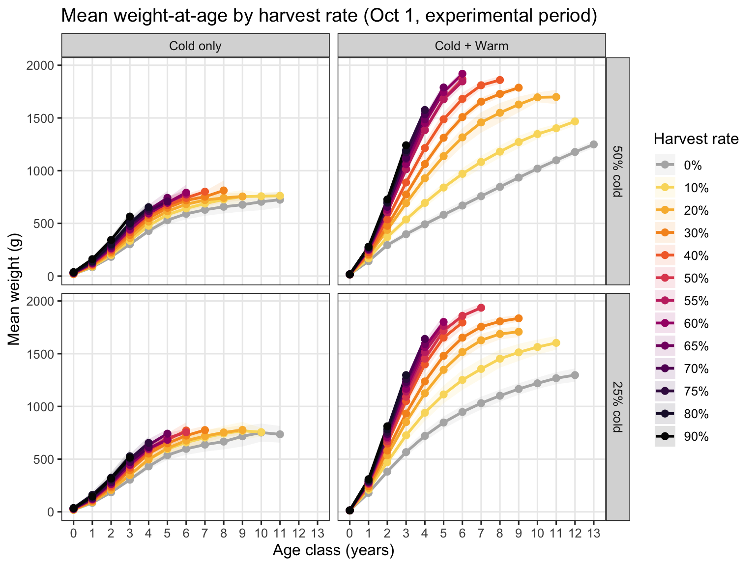
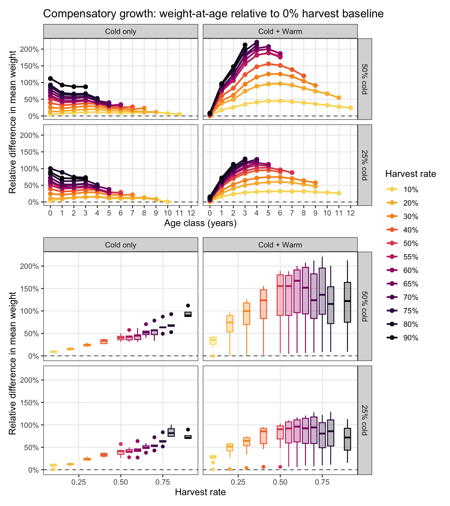
## Compensatory growth
```{r}
#| fig-width: 9
#| fig-height: 9
# Extract Oct 1 experimental-period rows, keyed by harvest rate.
# Filtering before bind_rows() keeps only ~1/365th of each data frame.
exp_oct1_hr <- purrr::map_dfr(ibm_list_mech, function(scen) {
  scen$oct1_exp |>
    mutate(hab_type = scen$ht,
           prop_cold = scen$pc,
           hr = scen$hr) %>%
    mutate(hab_type = factor(hab_type, levels = c("Cold only", "Cold + Warm")),
           prop_cold = factor(prop_cold, levels = pc_levels))
}) |>
  mutate(
    harvest_rate_fact = factor(hr_labels_mech[match(hr, hr_levels_mech)], levels = hr_labels_mech),
    prop_cold_fact = factor(pc_labels_mech[match(prop_cold, pc_levels_mech)], levels = pc_labels_mech)
  )

waa_hr <- exp_oct1_hr |>
  filter(yr >= 2060) %>% # filter b/c in some sim. runs it takes a few years for mean weight to stabilize following the start of harvest
  group_by(hab_type, prop_cold, prop_cold_fact, harvest_rate_fact, hr, age_class) |>
  summarise(
    mean_wt = mean(weight),
    sd_wt   = sd(weight),
    n       = n(),
    .groups = "drop"
  ) |>
  filter(n >= 10)

age_breaks_hr <- sort(unique(waa_hr$age_class))

p1 <- ggplot(waa_hr, aes(x = age_class, y = mean_wt,
                    color = harvest_rate_fact, fill = harvest_rate_fact)) +
  geom_ribbon(aes(ymin = pmax(0, mean_wt - sd_wt), ymax = mean_wt + sd_wt),
              alpha = 0.12, color = NA) +
  geom_line(linewidth = 1) +
  geom_point(size = 2.5, shape = 16) +
  scale_color_manual(values = hr_pal, name = "Harvest rate") +
  scale_fill_manual(values  = hr_pal, name = "Harvest rate") +
  scale_x_continuous(breaks = age_breaks_hr) +
  labs(
    x = "Age class (years)", y = "Mean weight (g)",
    title = "Mean weight-at-age by harvest rate (Oct 1, experimental period)"
  ) +
  theme_bw(base_size = 12) +
  theme(legend.position = "right", panel.grid.minor = element_blank()) +
  facet_grid(prop_cold_fact~hab_type)


# Relative difference vs. 0% harvest baseline
baseline_waa <- waa_hr |>
  filter(hr == 0) |>
  select(hab_type, prop_cold_fact, age_class, baseline_wt = mean_wt)

waa_hr_rd <- waa_hr |>
  filter(hr > 0) |>
  left_join(baseline_waa, by = c("hab_type", "prop_cold_fact", "age_class")) |>
  mutate(rel_diff = (mean_wt - baseline_wt) / baseline_wt)

p2 <- ggplot(waa_hr_rd, aes(x = age_class, y = rel_diff,
                       color = harvest_rate_fact, group = harvest_rate_fact)) +
  geom_hline(yintercept = 0, linetype = "dashed", color = "grey40") +
  geom_line(linewidth = 1) +
  geom_point(size = 2.5, shape = 16) +
  scale_color_manual(values = hr_pal, name = "Harvest rate") +
  scale_x_continuous(breaks = age_breaks_hr) +
  scale_y_continuous(labels = scales::label_percent(accuracy = 1)) +
  labs(
    x = "Age class (years)", y = "Relative difference in mean weight",
    title = "Compensatory growth: weight-at-age relative to 0% harvest baseline"
  ) +
  theme_bw(base_size = 12) +
  theme(panel.grid.minor = element_blank()) +
  facet_grid(prop_cold_fact~hab_type)


p3 <- ggplot(waa_hr_rd, aes(x = hr, y = rel_diff, color = harvest_rate_fact, fill = harvest_rate_fact, group = harvest_rate_fact)) +
  geom_hline(yintercept = 0, linetype = "dashed", color = "grey40") +
  # geom_line(linewidth = 1) +
  geom_boxplot() +
  scale_color_manual(values = hr_pal, name = "Harvest rate") +
  scale_fill_manual(values = scales::alpha(hr_pal, 0.3), name = "Harvest rate") +
  # scale_x_continuous(breaks = age_breaks_hr) +
  scale_y_continuous(labels = scales::label_percent(accuracy = 1)) +
  labs(
    x = "Harvest rate", y = "Relative difference in mean weight"
  ) +
  theme_bw(base_size = 12) +
  theme(legend.position = "none", panel.grid.minor = element_blank()) +
  facet_grid(prop_cold_fact~hab_type)

# (p1 / (p2 / p3 + plot_layout(axis_titles = "collect"))) + plot_layout(guides = "collect", heights = c(1.5, 2))
```
```{r}
#| fig-width: 8
#| fig-height: 6
p1
```
```{r}
#| fig-width: 8
#| fig-height: 9
(p2 + p3) + plot_layout(guides = "collect", heights = c(1.5, 2))
```
## Recruitment
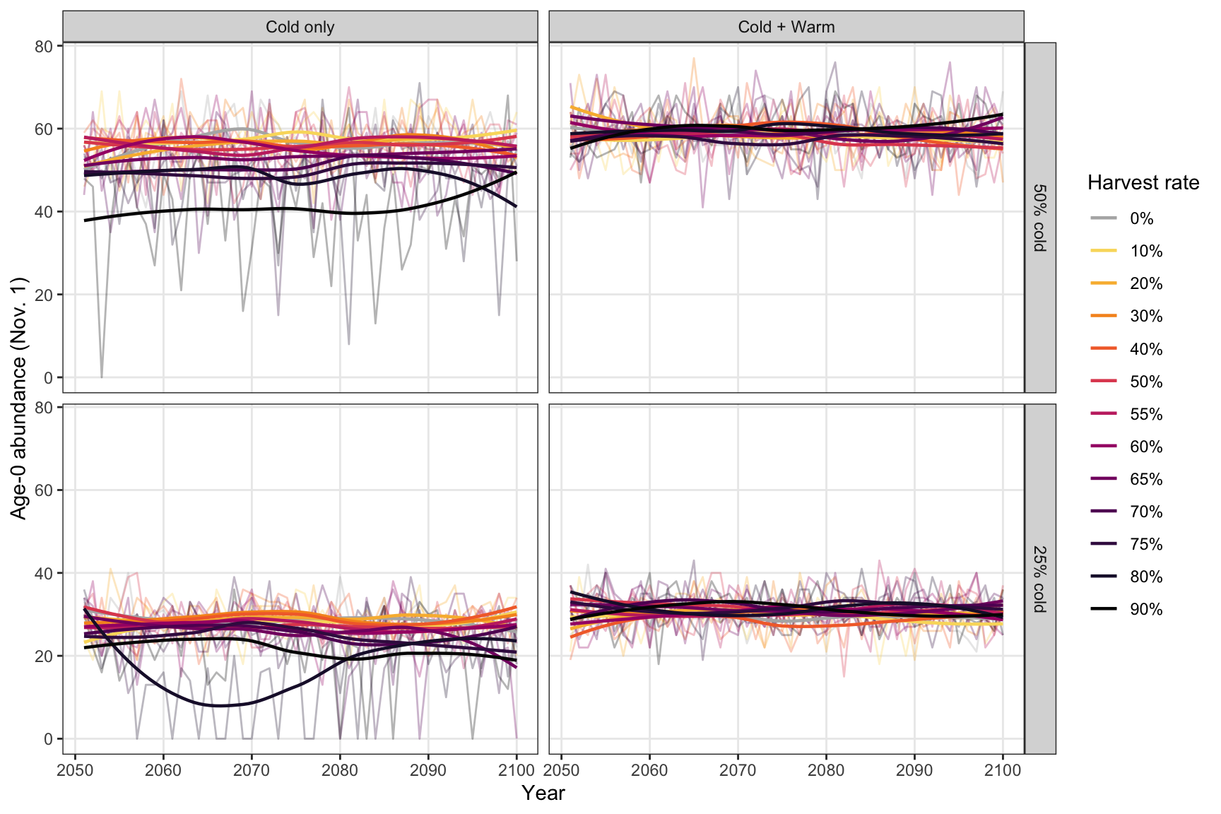
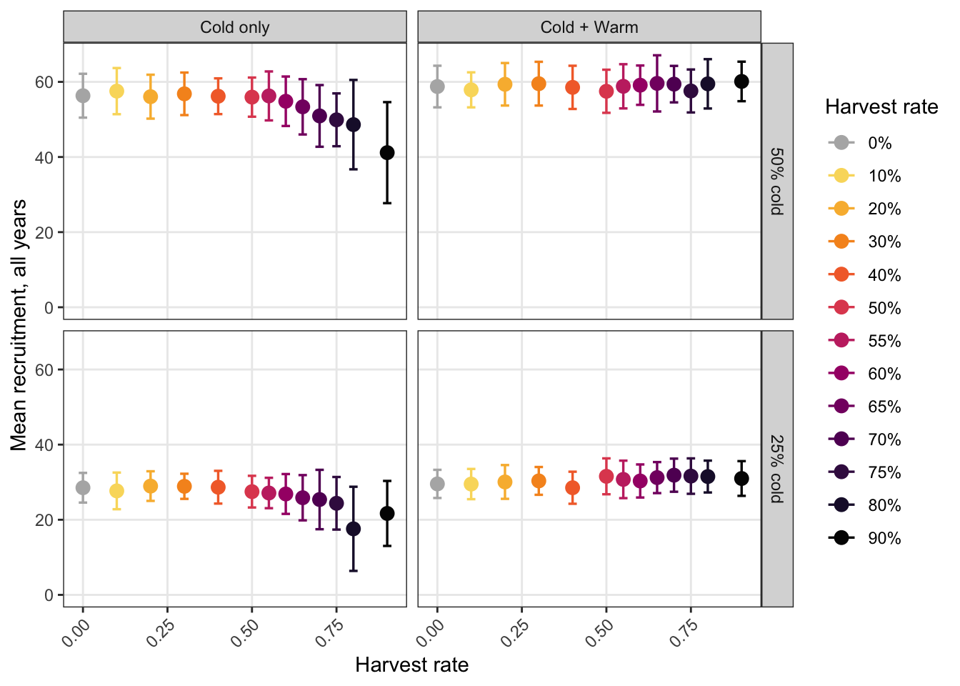
The number of fry produced is a function of adult size and abundance (fecundity), which are driven by warm and cold habitat availability. Importantly, when only cold habitat is available, the number of fry produced declines ~linearly with cold habitat availability. But when warm habitat is also available, considerably more fry are produced at a given proportion cold (except for 95% cold); i.e.,
```{r}
#| cache: false
# ── Annual age-0 recruitment time series ─────────────────────────────────────
# Zero-fill missing years so post-crash scenarios contribute zeros for the
# remainder of the experimental period rather than being silently excluded.
all_exp_years <- tibble(
  yr = seq(year(exp_start_date),
           year(exp_start_date) + base_params$nyears_experiment - 1L)
)

get_annual_age0 <- function(scen) {
  scen$age0_nov1 |>
    select(yr, n_age0) |>
    right_join(all_exp_years, by = "yr") |>
    replace_na(list(n_age0 = 0L)) |>
    mutate(
      hab_type          = scen$ht,
      prop_cold         = scen$pc,
      harvest_rate      = scen$hr,
      harvest_rate_fact = factor(scen$hr,
                                 levels = hr_levels_mech,
                                 labels = hr_labels_mech),
      hab_type          = factor(hab_type, levels = c("Cold only", "Cold + Warm")),
      prop_cold_fact    = factor(
        pc_labels_mech[match(scen$pc, pc_levels_mech)],
        levels = pc_labels_mech
      )
    )
}

age0_ts <- purrr::map_dfr(ibm_list_mech, get_annual_age0)


# ── End-vs-start recruitment ratio ───────────────────────────────────────────
# Collapses each trajectory to a single scalar: mean n_age0 in the last 10
# experimental years divided by the first 10. Stable harvest → ratio ≈ 1;
# slow decline → ratio < 1; crashed population → ratio = 0.
n_exp   <- nrow(all_exp_years)
first10 <- all_exp_years$yr[1:10]
last10  <- all_exp_years$yr[(n_exp - 9):n_exp]

ratio_df <- age0_ts |>
  mutate(period = case_when(
    yr %in% first10 ~ "start",
    yr %in% last10  ~ "end",
    TRUE            ~ NA_character_
  )) |>
  filter(!is.na(period)) |>
  group_by(hab_type, prop_cold, prop_cold_fact, harvest_rate, harvest_rate_fact, period) |>
  summarise(mean_n = mean(n_age0), sd_n = sd(n_age0), .groups = "drop") |>
  pivot_wider(names_from = period, values_from = c(mean_n, sd_n)) |>
  mutate(ratio = mean_n_end / mean_n_start) |>
  left_join(
    age0_ts |>
      group_by(hab_type, prop_cold, prop_cold_fact, harvest_rate, harvest_rate_fact) |>
      summarise(mean_n_all = mean(n_age0), sd_n_all = sd(n_age0), .groups = "drop"),
    by = c("hab_type", "prop_cold", "prop_cold_fact", "harvest_rate", "harvest_rate_fact")
  )
```
Age-0 abundance time series, faceted by habitat type and proportion cold habitat:
```{r}
#| fig-width: 9
#| fig-height: 6
ggplot(age0_ts, aes(x = yr, y = n_age0, color = harvest_rate_fact)) +
  geom_line(alpha = 0.3) +
  geom_smooth(linewidth = 0.8, se = FALSE) +
  scale_color_manual(values = hr_pal, name = "Harvest rate") +
  scale_x_continuous(name = "Year") +
  scale_y_continuous(name = "Age-0 abundance (Nov. 1)",
                     limits = c(0, NA),
                     labels = scales::label_comma()) +
  theme_bw() +
  theme(panel.grid.minor = element_blank()) +
  facet_grid(prop_cold_fact ~ hab_type)
```
Mean recruitment (all years), faceted by habitat type and proportion cold:
```{r}
#| fig-width: 7
#| fig-height: 5
ggplot(ratio_df, aes(x = harvest_rate, y = mean_n_all, color = harvest_rate_fact)) +
  geom_errorbar(aes(ymin = pmax(0, mean_n_all - sd_n_all), ymax = mean_n_all + sd_n_all),
                width = 0.025, linewidth = 0.6) +
  geom_point(size = 3) +
  scale_color_manual(values = hr_pal, name = "Harvest rate") +
  scale_y_continuous(name = "Mean recruitment, all years") +
  coord_cartesian(ylim = c(0, NA)) +
  labs(x = "Harvest rate") +
  theme_bw() +
  theme(panel.grid.minor = element_blank(),
        axis.text.x = element_text(angle = 45, hjust = 1)) +
  facet_grid(prop_cold_fact ~ hab_type)
```
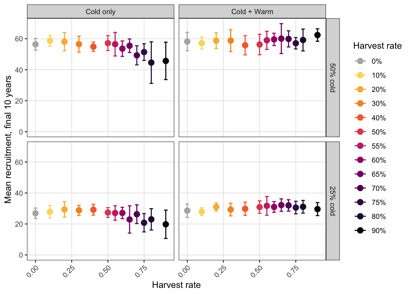
Mean recruitment over final 10 years, faceted by habitat type and proportion cold:
```{r}
#| fig-width: 7
#| fig-height: 5
ggplot(ratio_df, aes(x = harvest_rate, y = mean_n_end, color = harvest_rate_fact)) +
  geom_errorbar(aes(ymin = pmax(0, mean_n_end - sd_n_end), ymax = mean_n_end + sd_n_end),
                width = 0.025, linewidth = 0.6) +
  geom_point(size = 3) +
  scale_color_manual(values = hr_pal, name = "Harvest rate") +
  scale_y_continuous(name = "Mean recruitment, final 10 years",
                     limits = c(0, NA)) +
  labs(x = "Harvest rate") +
  theme_bw() +
  theme(panel.grid.minor = element_blank(),
        axis.text.x = element_text(angle = 45, hjust = 1)) +
  facet_grid(prop_cold_fact ~ hab_type)
```
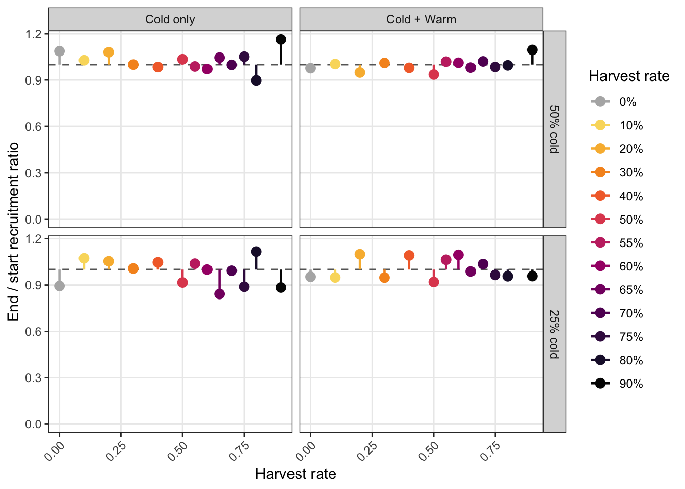
End/start recruitment ratio, faceted by habitat type and proportion cold:
```{r}
#| fig-width: 7
#| fig-height: 5
ggplot(ratio_df, aes(x = harvest_rate, y = ratio, color = harvest_rate_fact)) +
  geom_hline(yintercept = 1, linetype = "dashed", color = "grey40", linewidth = 0.6) +
  geom_segment(aes(xend = harvest_rate, yend = 1), linewidth = 0.8) +
  geom_point(size = 3) +
  scale_color_manual(values = hr_pal, name = "Harvest rate") +
  scale_y_continuous(name = "End / start recruitment ratio",
                     limits = c(0, NA)) +
  labs(x = "Harvest rate") +
  theme_bw() +
  theme(panel.grid.minor = element_blank(),
        axis.text.x = element_text(angle = 45, hjust = 1)) +
  facet_grid(prop_cold_fact ~ hab_type)
```
## Harvest
Summarize harvest data
```{r}
all_exp_years <- tibble(
  year = seq(year(exp_start_date),
           year(exp_start_date) + base_params$nyears_experiment - 1L)
)

get_annual_harvest <- function(scen) {
  scen$harvest %>%
    group_by(year) %>%
    summarise(n_harvested = n(),
              bm_harvested = sum(weight)/1000,
              mean_wt = mean(weight),
              sd_wt = sd(weight),
              mean_age = mean(age),
              sd_age = sd(age),
              mean_cond = mean(condition),
              sd_cond = sd(condition)) %>%
    ungroup() %>%
    right_join(all_exp_years, by = "year") %>%
    replace_na(list(n_harvested = 0L,
                    bm_harvested = 0L,
                    mean_wt = NA,
                    sd_wt = NA,
                    mean_age = NA,
                    sd_age = NA,
                    mean_cond = NA,
                    sd_cond = NA)) %>%
    mutate(hab_type = scen$ht,
           prop_cold = scen$pc,
           prop_cold_fact = factor(
             pc_labels_mech[match(scen$pc, pc_levels_mech)],
             levels = pc_labels_mech
           ),
           harvest_rate = scen$hr,
           harvest_rate_fact = factor(scen$hr,
                                      levels = hr_levels_mech,
                                      labels = hr_labels_mech))
}

get_harvest_traits <- function(scen) {
  scen$harvest %>%
    filter(year > 2060) %>%
    summarise(mean_wt = mean(weight),
              sd_wt = sd(weight),
              mean_age = mean(age),
              sd_age = sd(age),
              mean_cond = mean(condition),
              sd_cond = sd(condition)) %>%
    ungroup() %>%
    mutate(hab_type = scen$ht,
           prop_cold = scen$pc,
           prop_cold_fact = factor(
             pc_labels_mech[match(scen$pc, pc_levels_mech)],
             levels = pc_labels_mech
           ),
           harvest_rate = scen$hr,
           harvest_rate_fact = factor(scen$hr,
                                      levels = hr_levels_mech,
                                      labels = hr_labels_mech))
}


harvest_ts <- purrr::map_dfr(ibm_list_mech[c(2:13, 15:26, 28:39, 41:52)], get_annual_harvest) |>
  bind_rows(
    purrr::map_dfr(ibm_list_mech[c(1, 14, 27, 40)], function(scen) {
      tibble(
        year         = sort(unique(age0_ts$yr)),
        n_harvested  = 0L,
        bm_harvested = 0,
        mean_wt      = NA_real_,
        sd_wt        = NA_real_,
        mean_age     = NA_real_,
        sd_age       = NA_real_,
        mean_cond    = NA_real_,
        sd_cond      = NA_real_,
        hab_type     = scen$ht,
        prop_cold    = scen$pc,
        prop_cold_fact = factor(
          pc_labels_mech[match(scen$pc, pc_levels_mech)],
          levels = pc_labels_mech
        ),
        harvest_rate = scen$hr,
        harvest_rate_fact = factor(scen$hr,
                                   levels = hr_levels_mech,
                                   labels = hr_labels_mech)
      )
    })
  ) %>%
  mutate(hab_type = factor(hab_type, levels = c("Cold only", "Cold + Warm"))) %>%
  filter(year > 2060)

harvest_traits <- purrr::map_dfr(ibm_list_mech[c(2:13, 15:26, 28:39, 41:52)], get_harvest_traits) |>
  bind_rows(
    purrr::map_dfr(ibm_list_mech[c(1, 14, 27, 40)], function(scen) {
      tibble(
        mean_wt      = NA_real_,
        sd_wt        = NA_real_,
        mean_age     = NA_real_,
        sd_age       = NA_real_,
        mean_cond    = NA_real_,
        sd_cond      = NA_real_,
        hab_type     = scen$ht,
        prop_cold    = scen$pc,
        prop_cold_fact = factor(
          pc_labels_mech[match(scen$pc, pc_levels_mech)],
          levels = pc_labels_mech
        ),
        harvest_rate = scen$hr,
        harvest_rate_fact = factor(scen$hr,
                                   levels = hr_levels_mech,
                                   labels = hr_labels_mech)
      )
    })
  ) %>%
  mutate(hab_type = factor(hab_type, levels = c("Cold only", "Cold + Warm")))


harvest_summ <- harvest_ts %>%
  group_by(hab_type, prop_cold, prop_cold_fact, harvest_rate, harvest_rate_fact) %>%
  summarize(mean_n = mean(n_harvested),
            sd_n = sd(n_harvested),
            mean_bm = mean(bm_harvested),
            sd_bm = sd(bm_harvested)) %>%
  ungroup() %>%
  left_join(harvest_traits,
            by = c("hab_type", "prop_cold", "prop_cold_fact",
                   "harvest_rate", "harvest_rate_fact"))
```
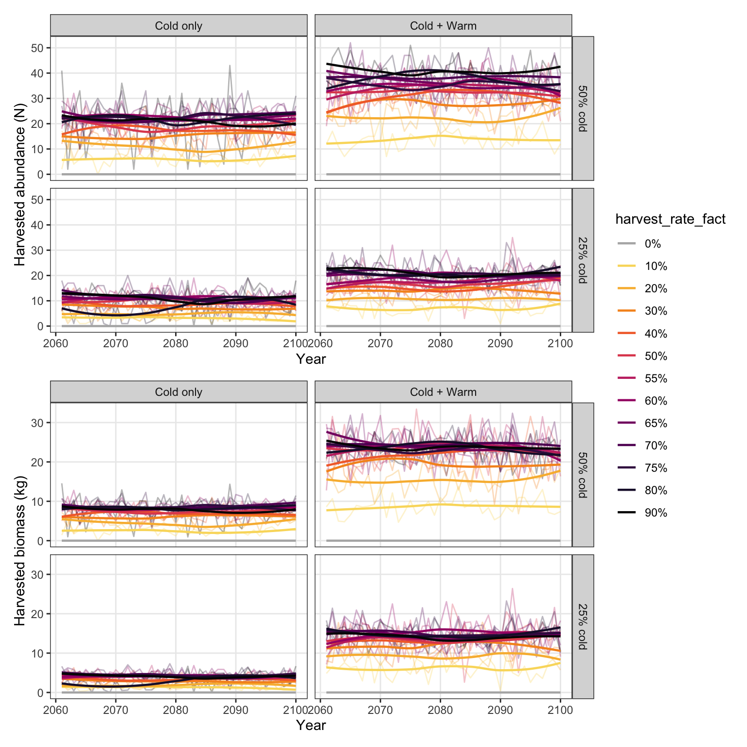
Show time series of harvested abundance, by habitat configuration and harvest rate
```{r}
#| cache: false
#| fig-width: 8
#| fig-height: 8
p1 <- ggplot(harvest_ts, aes(x = year, y = n_harvested, color = harvest_rate_fact)) +
  geom_line(alpha = 0.3) +
  geom_smooth(linewidth = 0.8, se = FALSE) +
  scale_color_manual(values = hr_pal) +
  # coord_cartesian(ylim = c(0, 90)) +
  labs(x = "Year", y = "Harvested abundance (N)") +
  theme_bw() +
  theme(panel.grid.minor = element_blank()) +
  facet_grid(prop_cold_fact ~ hab_type)

p2 <- ggplot(harvest_ts, aes(x = year, y = bm_harvested, color = harvest_rate_fact)) +
  geom_line(alpha = 0.3) +
  geom_smooth(linewidth = 0.8, se = FALSE) +
  scale_color_manual(values = hr_pal) +
  # coord_cartesian(ylim = c(0, 50)) +
  labs(x = "Year", y = "Harvested biomass (kg)") +
  theme_bw() +
  theme(panel.grid.minor = element_blank()) +
  facet_grid(prop_cold_fact ~ hab_type)

(p1 / p2) + plot_layout(guides = "collect")
```
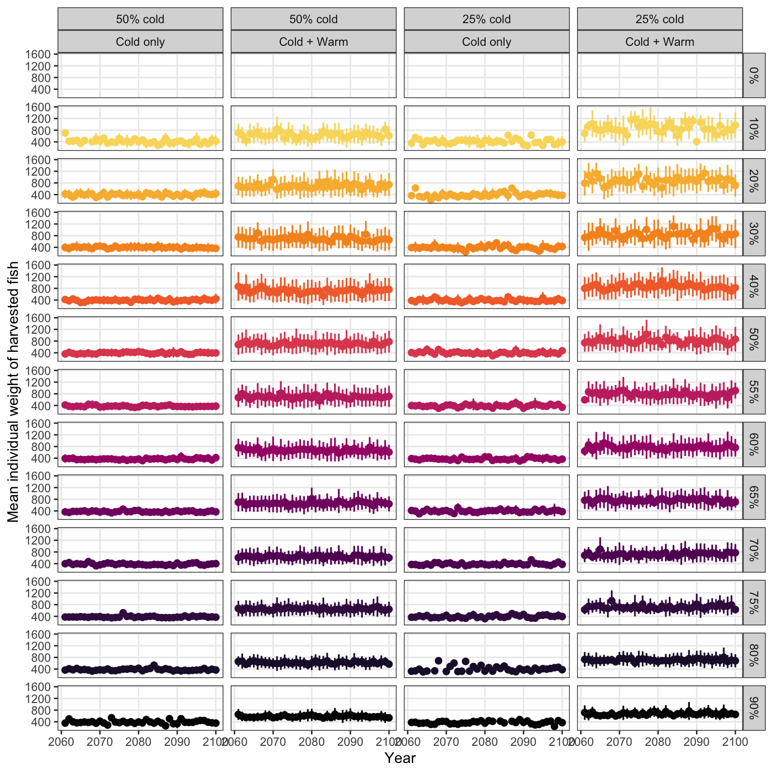
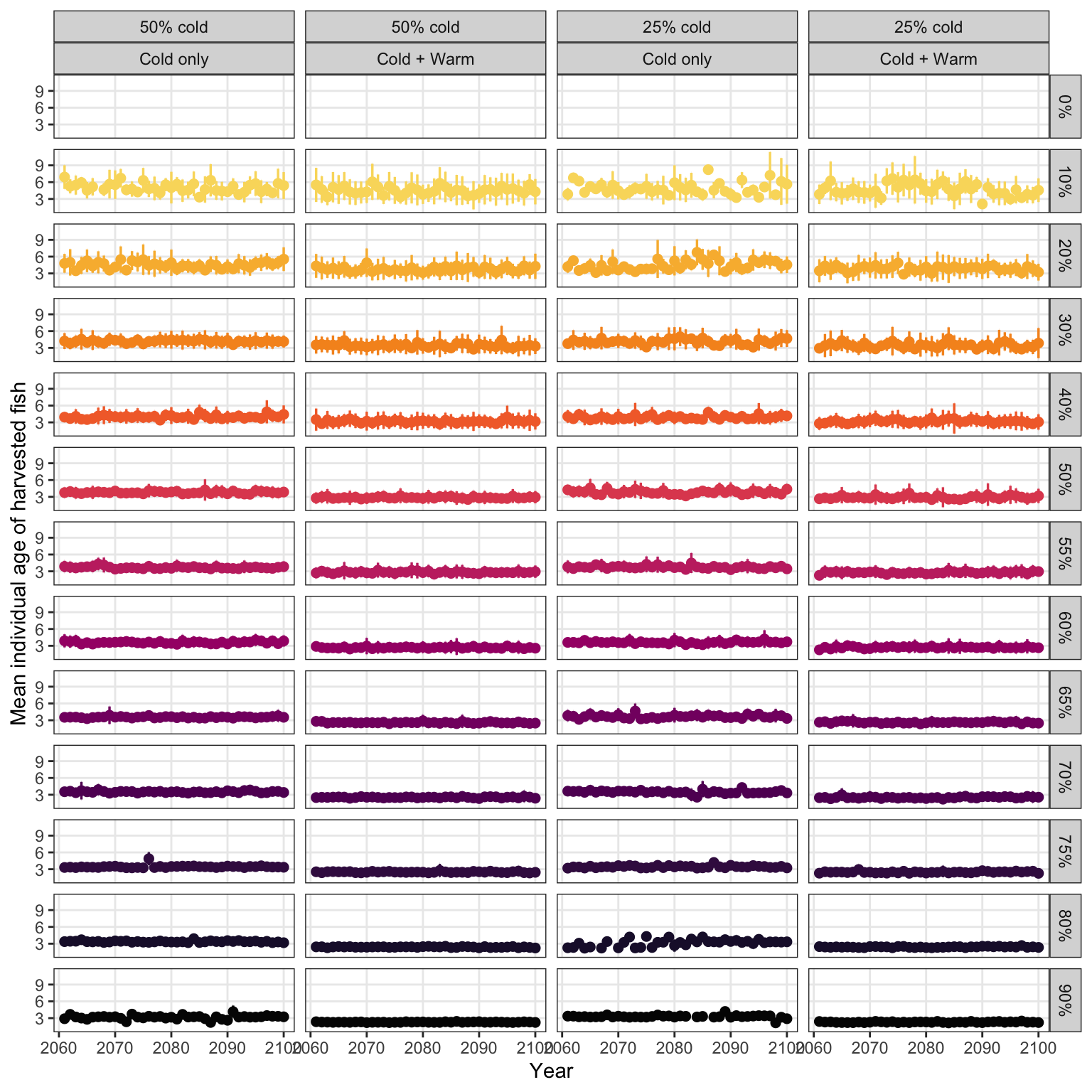
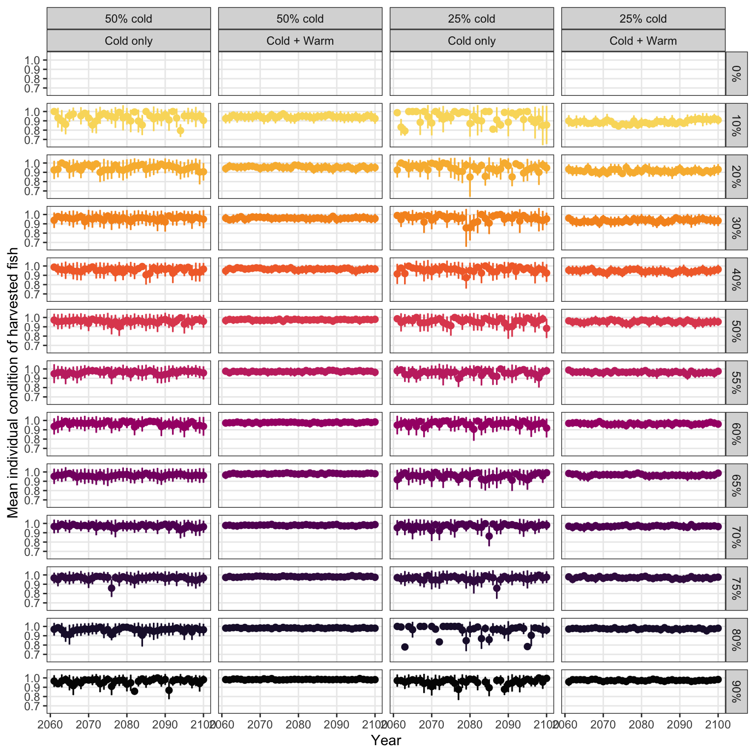
Time series of individual-level traits
::: {.panel-tabset}
### Weight
```{r}
#| cache: false
#| fig-width: 8
#| fig-height: 8
ggplot(harvest_ts, aes(x = year, y = mean_wt, color = harvest_rate_fact)) +
  geom_errorbar(aes(ymin = mean_wt - sd_wt, ymax = mean_wt + sd_wt), width = 0.025, linewidth = 0.6) +
  geom_point(size = 2) +
  facet_grid(harvest_rate_fact ~ prop_cold_fact + hab_type) +
  scale_color_manual(values = hr_pal, guide = "none") +
  labs(x = "Year", y = "Mean individual weight of harvested fish") +
  theme_bw() +
  theme(panel.grid.minor = element_blank())
```
### Age
```{r}
#| cache: false
#| fig-width: 8
#| fig-height: 8
ggplot(harvest_ts, aes(x = year, y = mean_age, color = harvest_rate_fact)) +
  geom_errorbar(aes(ymin = mean_age - sd_age, ymax = mean_age + sd_age), width = 0.025, linewidth = 0.6) +
  geom_point(size = 2) +
  facet_grid(harvest_rate_fact ~ prop_cold_fact + hab_type) +
  scale_color_manual(values = hr_pal, guide = "none") +
  labs(x = "Year", y = "Mean individual age of harvested fish") +
  theme_bw() +
  theme(panel.grid.minor = element_blank())
```
### Condition
```{r}
#| cache: false
#| fig-width: 8
#| fig-height: 8
ggplot(harvest_ts, aes(x = year, y = mean_cond, color = harvest_rate_fact)) +
  geom_errorbar(aes(ymin = mean_cond - sd_cond, ymax = mean_cond + sd_cond), width = 0.025, linewidth = 0.6) +
  geom_point(size = 2) +
  facet_grid(harvest_rate_fact ~ prop_cold_fact + hab_type) +
  scale_color_manual(values = hr_pal, guide = "none") +
  labs(x = "Year", y = "Mean individual condition of harvested fish") +
  theme_bw() +
  theme(panel.grid.minor = element_blank())
```
:::
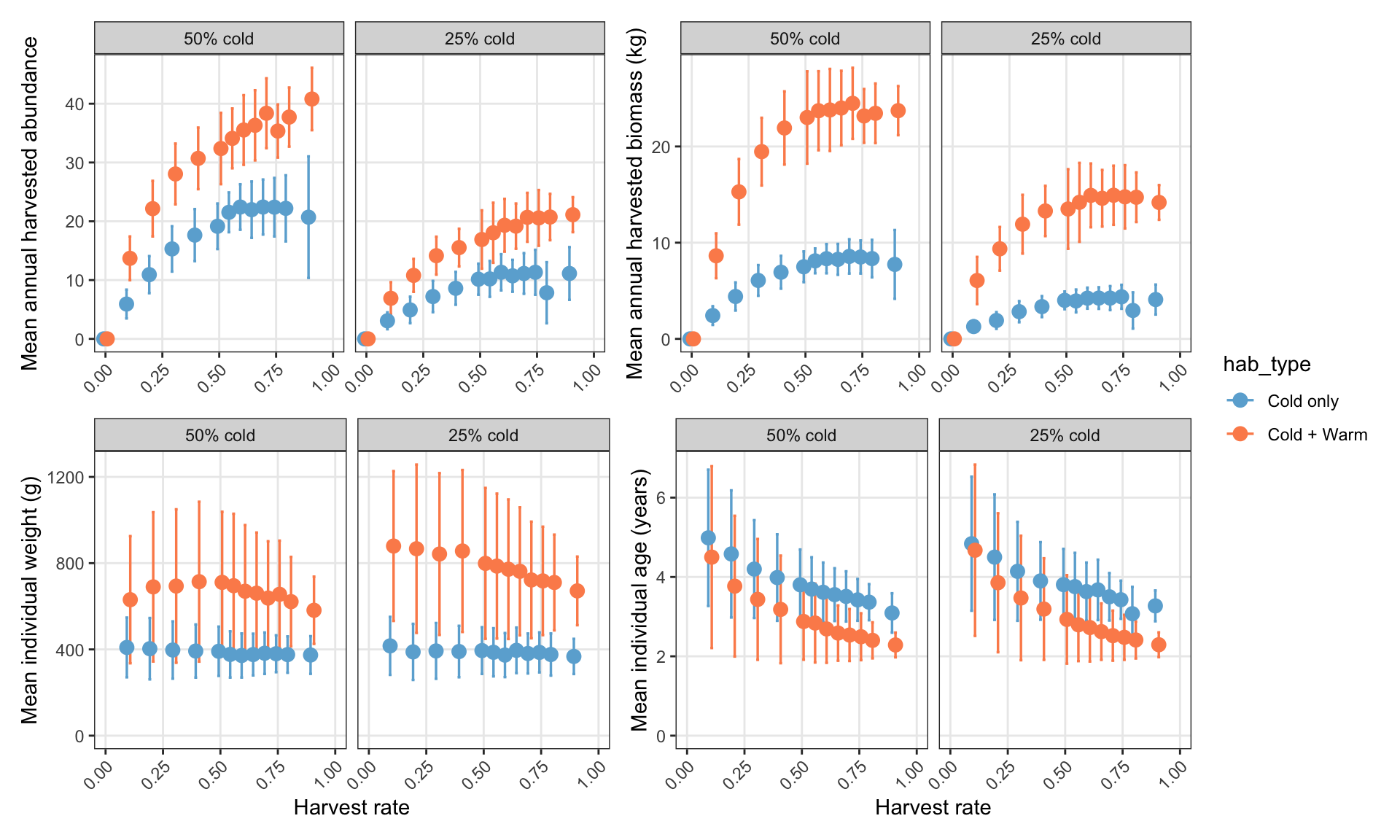
```{r}
#| cache: false
#| fig-width: 10
#| fig-height: 6
# mean harvested abundance
p_abun <- ggplot(harvest_summ, aes(x = harvest_rate, y = mean_n, color = hab_type, group = hab_type)) +
  geom_errorbar(aes(ymin = mean_n - sd_n, ymax = mean_n + sd_n), width = 0.025, linewidth = 0.6, position = position_dodge(width = 0.03)) +
  geom_point(size = 3, position = position_dodge(width = 0.03)) +
  scale_color_manual(values = hab_cols) +
  scale_y_continuous(name = "Mean annual harvested abundance") +
  coord_cartesian(xlim = c(0,1), ylim = c(0,NA)) +
  labs(x = "Harvest rate") +
  theme_bw() +
  theme(panel.grid.minor = element_blank(),
        axis.text.x      = element_text(angle = 45, hjust = 1),
        axis.title.x = element_blank()) +
  facet_wrap(~prop_cold_fact)

# mean harvested biomass
p_biom <- ggplot(harvest_summ, aes(x = harvest_rate, y = mean_bm, color = hab_type, group = hab_type)) +
  geom_errorbar(aes(ymin = mean_bm - sd_bm, ymax = mean_bm + sd_bm), width = 0.025, linewidth = 0.6, position = position_dodge(width = 0.03)) +
  geom_point(size = 3, position = position_dodge(width = 0.03)) +
  scale_color_manual(values = hab_cols) +
  scale_y_continuous(name = "Mean annual harvested biomass (kg)") +
  coord_cartesian(xlim = c(0,1), ylim = c(0,NA)) +
  labs(x = "Harvest rate") +
  theme_bw() +
  theme(panel.grid.minor = element_blank(),
        axis.text.x      = element_text(angle = 45, hjust = 1),
        axis.title.x = element_blank()) +
  facet_wrap(~prop_cold_fact)

# mean individual weight
p_wt <- ggplot(harvest_summ, aes(x = harvest_rate, y = mean_wt, color = hab_type, group = hab_type)) +
  geom_errorbar(aes(ymin = mean_wt - sd_wt, ymax = mean_wt + sd_wt), width = 0.025, linewidth = 0.6, position = position_dodge(width = 0.03)) +
  geom_point(size = 3, position = position_dodge(width = 0.03)) +
  scale_color_manual(values = hab_cols) +
  scale_y_continuous(name = "Mean individual weight (g)") +
  coord_cartesian(xlim = c(0,1), ylim = c(0,NA)) +
  labs(x = "Harvest rate") +
  theme_bw() +
  theme(panel.grid.minor = element_blank(),
        axis.text.x      = element_text(angle = 45, hjust = 1)) +
  facet_wrap(~prop_cold_fact)

# mean individual age
p_age <- ggplot(harvest_summ, aes(x = harvest_rate, y = mean_age, color = hab_type, group = hab_type)) +
  geom_errorbar(aes(ymin = mean_age - sd_age, ymax = mean_age + sd_age), width = 0.025, linewidth = 0.6, position = position_dodge(width = 0.03)) +
  geom_point(size = 3, position = position_dodge(width = 0.03)) +
  scale_color_manual(values = hab_cols) +
  scale_y_continuous(name = "Mean individual age (years)") +
  coord_cartesian(xlim = c(0,1), ylim = c(0,NA)) +
  labs(x = "Harvest rate") +
  theme_bw() +
  theme(panel.grid.minor = element_blank(),
        axis.text.x      = element_text(angle = 45, hjust = 1)) +
  facet_wrap(~prop_cold_fact)


(p_abun + p_biom) / (p_wt + p_age) + plot_layout(guides = "collect")
```
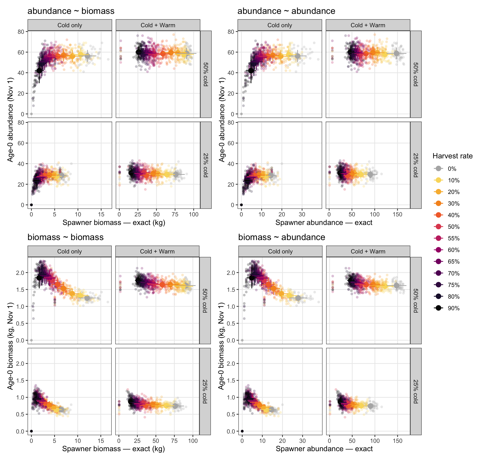
## Adult-to-juvenile stock-recruitment
Two measures of spawner biomass are compared: (1) the exact biomass recorded in the spawn log (sum of unique spawner weights per year), and (2) an estimate from the IBM state on April 15 — the total weight of all surviving fish heavier than 200 g just before the spawning window opens. Recruitment is age-0 abundance and biomass on November 1.
```{r}
#| cache: false
#| fig-width: 10
#| fig-height: 9.5
# Local year grid (avoids depending on the column name of the global all_exp_years,
# which is redefined with a different name later in the document).
sr_exp_years <- tibble(yr = seq(year(exp_start_date),
                                year(exp_start_date) + base_params$nyears_experiment - 1L))

# ── Annual spawner biomass from spawn_log ─────────────────────────────────────
# Each parent may appear more than once per year (multiple spawning attempts);
# average their weight within year before summing to avoid double-counting mass.
get_annual_spawner_log <- function(scen) {
  scen$spawn_log |>
    mutate(date = base_params$mindate + (dayofsim - 1L),
           yr   = year(date)) |>
    filter(date >= exp_start_date) |>
    group_by(yr, parent_pid) |>
    summarise(parent_wt = mean(weight), .groups = "drop") |>
    group_by(yr) |>
    summarise(spawn_biom_log = sum(parent_wt),
              n_spawners     = n_distinct(parent_pid),
              .groups = "drop") |>
    right_join(sr_exp_years, by = "yr") |>
    replace_na(list(spawn_biom_log = 0, n_spawners = 0L)) |>
    mutate(hab_type          = scen$ht,
           prop_cold         = scen$pc,
           prop_cold_fact    = factor(
             pc_labels_mech[match(scen$pc, pc_levels_mech)],
             levels = pc_labels_mech
           ),
           harvest_rate      = scen$hr,
           harvest_rate_fact = factor(scen$hr,
                                      levels = hr_levels_mech,
                                      labels = hr_labels_mech)) %>%
    mutate(hab_type = factor(hab_type, levels = c("Cold only", "Cold + Warm")))
}

spawner_log_ts <- purrr::map_dfr(ibm_list_mech, get_annual_spawner_log)


# ── Age-0 recruitment: abundance and biomass on November 1 ────────────────────
get_annual_recruit <- function(scen) {
  scen$age0_nov1 |>
    right_join(sr_exp_years, by = "yr") |>
    replace_na(list(n_age0 = 0L, biom_age0 = 0)) |>
    mutate(hab_type          = scen$ht,
           prop_cold         = scen$pc,
           prop_cold_fact    = factor(
             pc_labels_mech[match(scen$pc, pc_levels_mech)],
             levels = pc_labels_mech
           ),
           harvest_rate      = scen$hr,
           harvest_rate_fact = factor(scen$hr,
                                      levels = hr_levels_mech,
                                      labels = hr_labels_mech)) %>%
    mutate(hab_type = factor(hab_type, levels = c("Cold only", "Cold + Warm")))
}

recruit_ts <- purrr::map_dfr(ibm_list_mech, get_annual_recruit)

# ── Join into one SR data frame ───────────────────────────────────────────────
sr_ts <- recruit_ts |>
  left_join(
    spawner_log_ts |>
      select(hab_type, prop_cold, yr, harvest_rate, spawn_biom_log, n_spawners),
    by = c("hab_type", "prop_cold", "yr", "harvest_rate")
  ) |>
  # left_join(spawner_apr_ts |> select(yr, harvest_rate, spawn_biom_apr, n_spawn_elig),
  #           by = c("yr", "harvest_rate")) %>%
  mutate(prod_nb = log(n_age0 / spawn_biom_log))

# Per-scenario means and SDs (collapsed across years)
sr_summ <- sr_ts |>
  filter(!is.na(prod_nb)) %>%
  group_by(hab_type, prop_cold, prop_cold_fact, harvest_rate, harvest_rate_fact) |>
  summarise(
    across(c(n_age0, biom_age0, spawn_biom_log, n_spawners, prod_nb),
           list(mean = mean, sd = sd)),
    .groups = "drop"
  )

# ── Plots ─────────────────────────────────────────────────────────────────────
# Convert biomass to kg for readability
kg <- function(x) x / 1000

# Helper: one SR panel. Uses inherit.aes = FALSE on summary layers to avoid
# the global aes (which maps sr_ts columns) being applied to sr_summ data.
# x_kg / y_kg: set TRUE to divide that axis by 1000 (g -> kg); FALSE for counts.
sr_panel <- function(x_raw, y_raw, x_summ, y_summ,
                     x_sd_summ, y_sd_summ, x_lab, y_lab, title,
                     x_kg = FALSE, y_kg = FALSE) {
  x_fn <- if (x_kg) kg else identity
  y_fn <- if (y_kg) kg else identity
  ggplot(sr_ts, aes(x = x_fn({{ x_raw }}), y = y_fn({{ y_raw }}),
                    color = harvest_rate_fact)) +
    geom_point(alpha = 0.25, size = 1.5, shape = 16) +
    geom_point(data = sr_summ, inherit.aes = FALSE,
               aes(x = x_fn({{ x_summ }}), y = y_fn({{ y_summ }}),
                   color = harvest_rate_fact),
               size = 3.5, shape = 16) +
    # vertical error bars (recruitment uncertainty)
    geom_errorbar(data = sr_summ, inherit.aes = FALSE,
                  aes(x = x_fn({{ x_summ }}),
                      ymin = pmax(0, y_fn({{ y_summ }}) - y_fn({{ y_sd_summ }})),
                      ymax = y_fn({{ y_summ }}) + y_fn({{ y_sd_summ }}),
                      color = harvest_rate_fact),
                  width = 0, linewidth = 0.5) +
    # horizontal error bars (spawner uncertainty)
    geom_segment(data = sr_summ, inherit.aes = FALSE,
                 aes(x    = pmax(0, x_fn({{ x_summ }}) - x_fn({{ x_sd_summ }})),
                     xend = x_fn({{ x_summ }}) + x_fn({{ x_sd_summ }}),
                     y    = y_fn({{ y_summ }}),
                     yend = y_fn({{ y_summ }}),
                     color = harvest_rate_fact),
                 linewidth = 0.5) +
    scale_color_manual(values = hr_pal, name = "Harvest rate") +
    scale_x_continuous(labels = scales::label_comma()) +
    scale_y_continuous(labels = scales::label_comma(), limits = c(0, NA)) +
    labs(x = x_lab, y = y_lab, title = title) +
    theme_bw(base_size = 11) +
    theme(panel.grid.minor = element_blank(), legend.position = "none") +
    facet_grid(prop_cold_fact ~ hab_type, scales = "free_x")
}

p_sr_1 <- sr_panel(
  x_raw = spawn_biom_log,       y_raw = n_age0,
  x_summ = spawn_biom_log_mean, y_summ = n_age0_mean,
  x_sd_summ = spawn_biom_log_sd, y_sd_summ = n_age0_sd,
  x_lab = "Spawner biomass — exact (kg)", y_lab = "Age-0 abundance (Nov 1)",
  title = "abundance ~ biomass",
  x_kg = TRUE, y_kg = FALSE
)

p_sr_2 <- sr_panel(
  x_raw = spawn_biom_log,       y_raw = biom_age0,
  x_summ = spawn_biom_log_mean, y_summ = biom_age0_mean,
  x_sd_summ = spawn_biom_log_sd, y_sd_summ = biom_age0_sd,
  x_lab = "Spawner biomass — exact (kg)", y_lab = "Age-0 biomass (kg, Nov 1)",
  title = "biomass ~ biomass",
  x_kg = TRUE, y_kg = TRUE
)

p_sr_3 <- sr_panel(
  x_raw = n_spawners,       y_raw = n_age0,
  x_summ = n_spawners_mean, y_summ = n_age0_mean,
  x_sd_summ = n_spawners_sd, y_sd_summ = n_age0_sd,
  x_lab = "Spawner abundance — exact", y_lab = "Age-0 abundance (Nov 1)",
  title = "abundance ~ abundance",
  x_kg = FALSE, y_kg = FALSE
)

p_sr_4 <- sr_panel(
  x_raw = n_spawners,       y_raw = biom_age0,
  x_summ = n_spawners_mean, y_summ = biom_age0_mean,
  x_sd_summ = n_spawners_sd, y_sd_summ = biom_age0_sd,
  x_lab = "Spawner abundance — exact", y_lab = "Age-0 biomass (kg, Nov 1)",
  title = "biomass ~ abundance",
  x_kg = FALSE, y_kg = TRUE
)

(p_sr_1 + p_sr_3) / (p_sr_2 + p_sr_4) +
  plot_layout(guides = "collect") &
  theme(legend.position = "right")
```
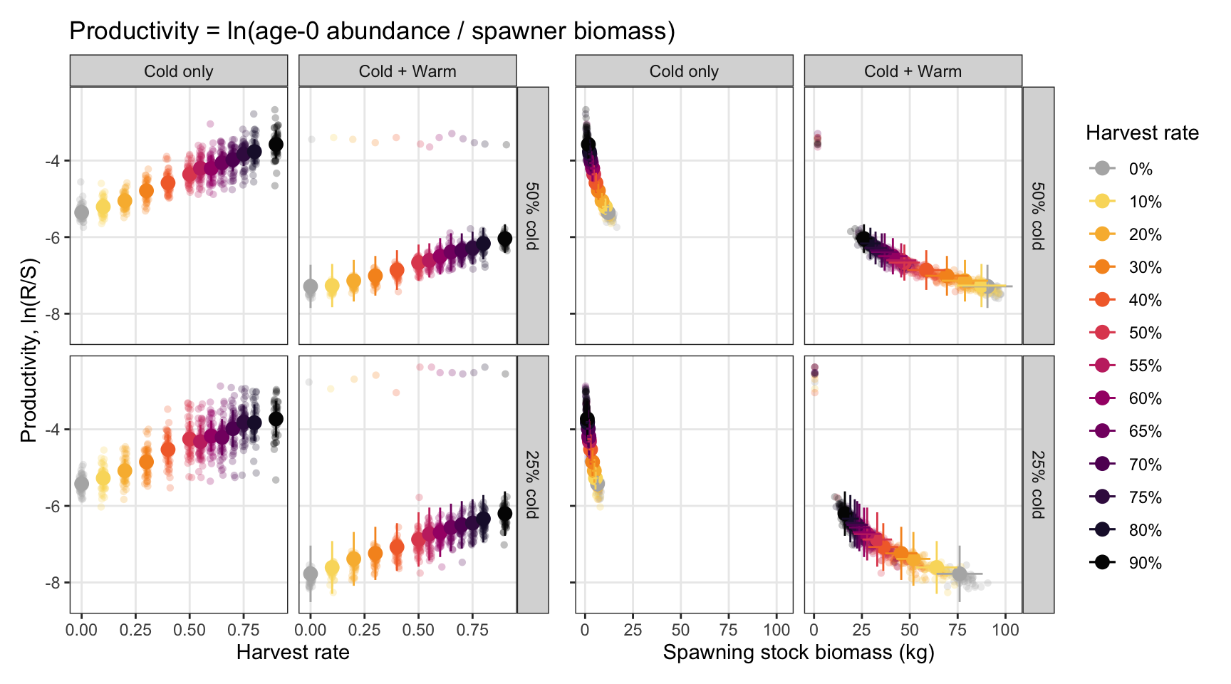
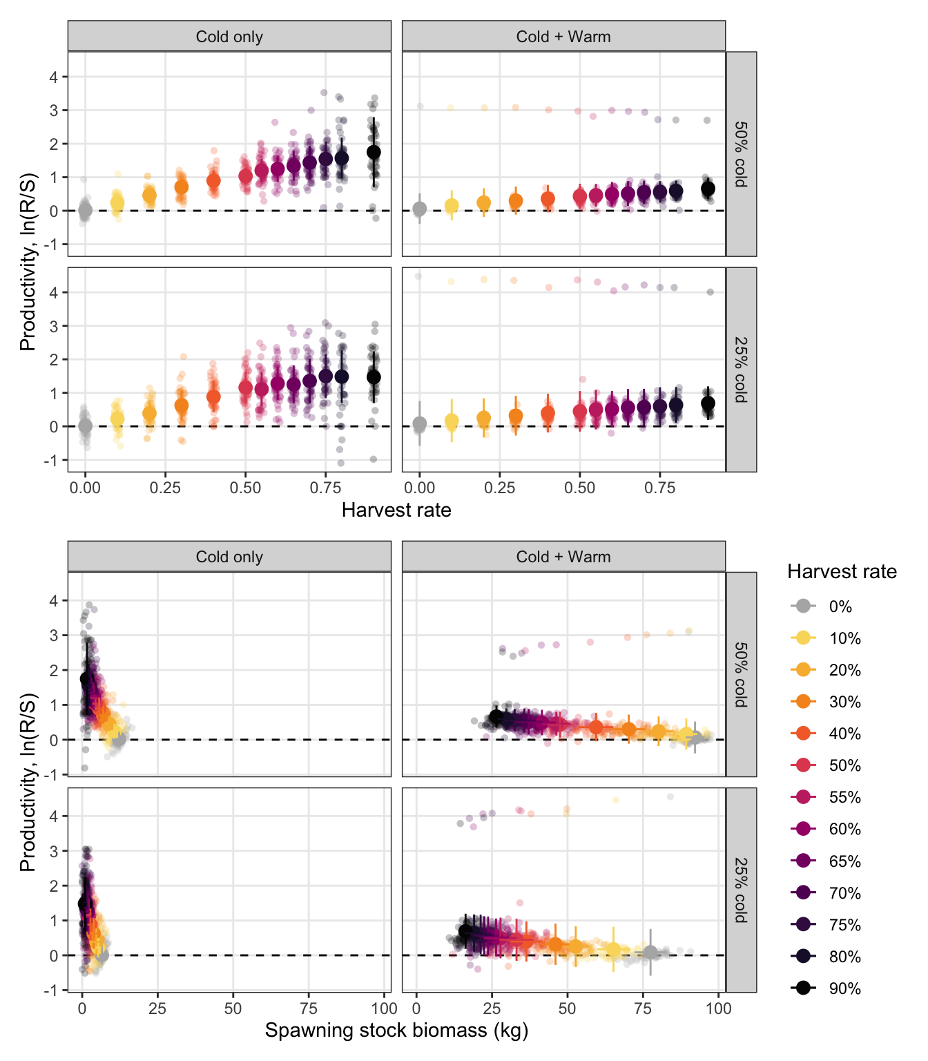
Inspect relationships between productivity (logged recruits per spawner) and harvest rate and spawning stock biomass.
```{r}
#| cache: false
#| fig-width: 9
#| fig-height: 5
p1 <- sr_ts %>%
  ggplot(aes(x = jitter(harvest_rate), y = prod_nb, color = harvest_rate_fact)) +
  geom_point(alpha = 0.25, size = 1.5, shape = 16) +
  geom_point(data = sr_summ, inherit.aes = FALSE, size = 3,
             aes(x = harvest_rate, y = prod_nb_mean, color = harvest_rate_fact)) +
  geom_errorbar(data = sr_summ, inherit.aes = FALSE,
                aes(x = harvest_rate, ymin = prod_nb_mean - prod_nb_sd, ymax = prod_nb_mean + prod_nb_sd, color = harvest_rate_fact),
                width = 0, linewidth = 0.5) +
  scale_color_manual(values = hr_pal, name = "Harvest rate") +
  # scale_x_continuous(labels = scales::label_comma()) +
  # scale_y_continuous(labels = scales::label_comma(), limits = c(0, NA)) +
  labs(x = "Harvest rate", y = "Productivity, ln(R/S)", title = "Productivity = ln(age-0 abundance / spawner biomass)") +
  theme_bw(base_size = 11) +
  theme(panel.grid.minor = element_blank(), legend.position = "none") +
  facet_grid(prop_cold_fact ~ hab_type)


p2 <- sr_ts %>%
  ggplot(aes(x = spawn_biom_log/1000, y = prod_nb, color = harvest_rate_fact)) +
  geom_point(alpha = 0.25, size = 1.5, shape = 16) +
  geom_point(data = sr_summ, inherit.aes = FALSE, size = 3,
             aes(x = spawn_biom_log_mean/1000, y = prod_nb_mean, color = harvest_rate_fact)) +
  geom_errorbar(data = sr_summ, inherit.aes = FALSE,
                aes(x = spawn_biom_log_mean/1000, ymin = prod_nb_mean - prod_nb_sd, ymax = prod_nb_mean + prod_nb_sd, color = harvest_rate_fact),
                width = 0, linewidth = 0.5) +
  geom_segment(data = sr_summ, inherit.aes = FALSE,
               aes(x = spawn_biom_log_mean/1000 - spawn_biom_log_sd/1000, xend = spawn_biom_log_mean/1000 + spawn_biom_log_sd/1000,
                   y = prod_nb_mean, yend = prod_nb_mean,
                   color = harvest_rate_fact)) +
  scale_color_manual(values = hr_pal, name = "Harvest rate") +
  # scale_x_continuous(labels = scales::label_comma()) +
  # scale_y_continuous(labels = scales::label_comma(), limits = c(0, NA)) +
  labs(x = "Spawning stock biomass (kg)", y = "Productivity, ln(R/S)") +
  theme_bw(base_size = 11) +
  theme(panel.grid.minor = element_blank(), legend.position = "none", axis.text.y = element_blank(), axis.title.y = element_blank()) +
  facet_grid(prop_cold_fact ~ hab_type)

(p1 + p2) +
  # plot_layout(guides = "collect") &
  theme(legend.position = "right")
```
## Adult-to-adult stock-recruitment
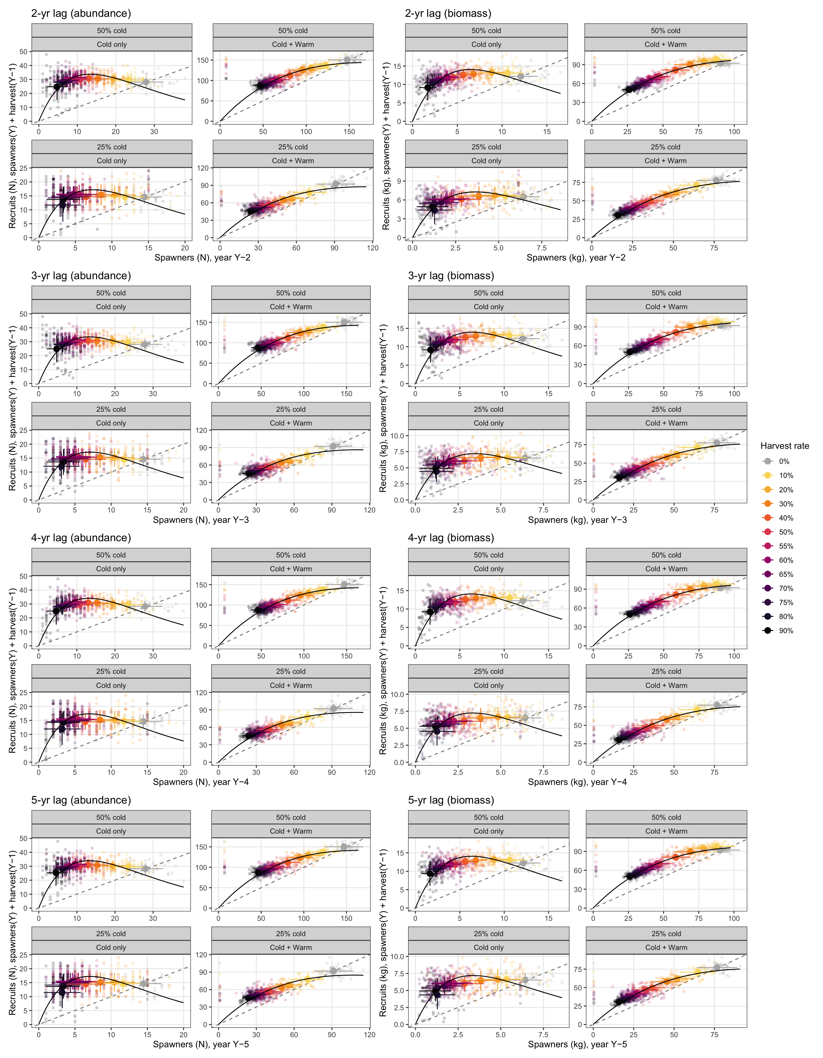
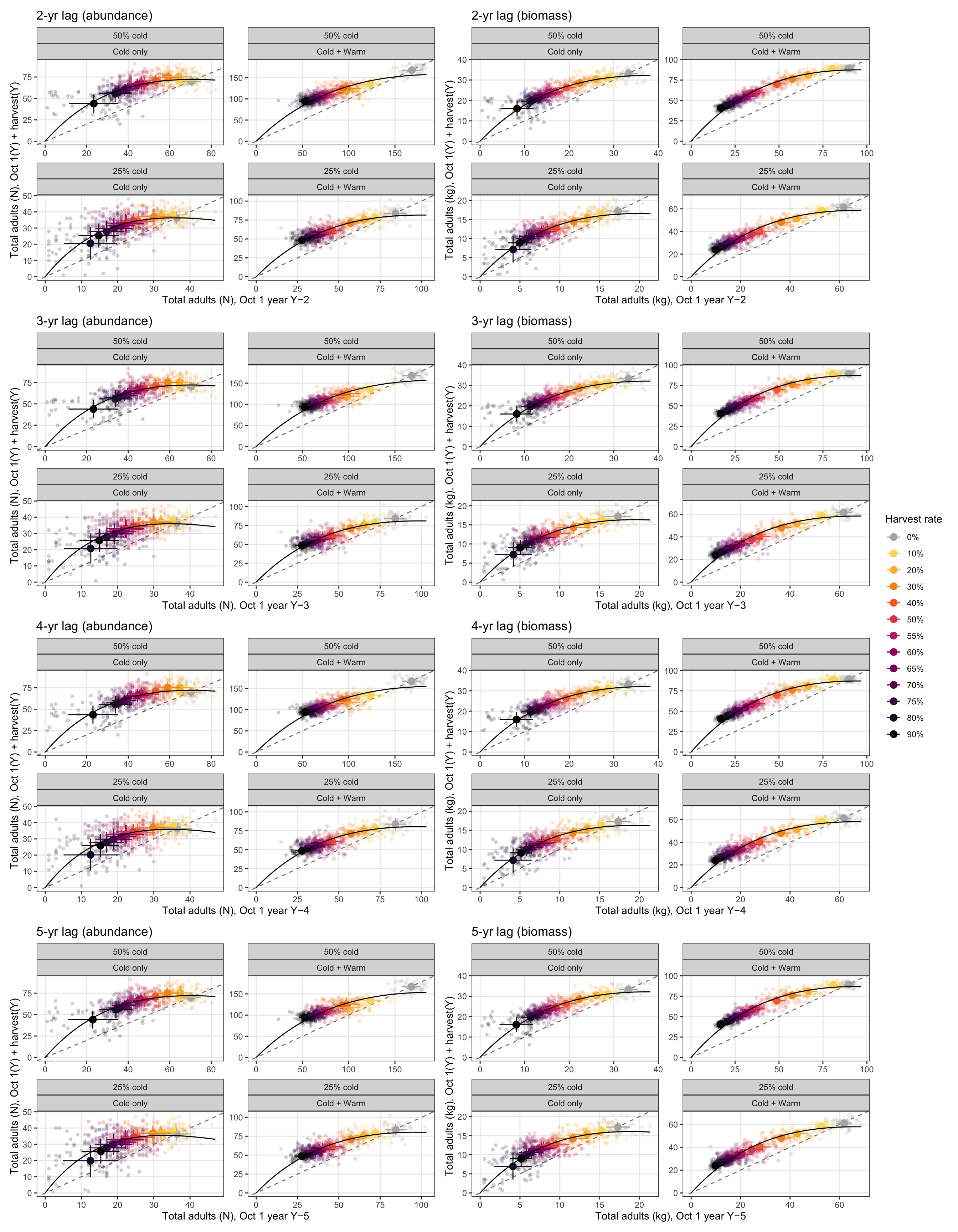
Recruitment is expressed as the number of adults that survived to spawning size in year Y, defined as spawners(Y) + fish harvested in summer Y−1 (those that would have spawned but were removed). This is paired with the parent spawning stock 3 years earlier (minimum age at maturity), and compared to the 1:1 replacement line to identify surplus production.
### Spawner based
#### Derive stock-recruitment curves
Derive adult-to-adult stock-recruitment curves over 4 different lag periods (2-5 years), for abundance and biomass separately.
```{r}
#| fig-width: 14
#| fig-height: 18
# ── Annual harvest abundance and biomass per scenario ─────────────────────────
get_annual_harvest_nb <- function(scen) {
  base_cols <- list(
    hab_type       = scen$ht,
    prop_cold      = scen$pc,
    prop_cold_fact = factor(
      pc_labels_mech[match(scen$pc, pc_levels_mech)],
      levels = pc_labels_mech
    ),
    harvest_rate      = scen$hr,
    harvest_rate_fact = factor(scen$hr,
                               levels = hr_levels_mech,
                               labels = hr_labels_mech)
  )
  if (is.null(scen$harvest)) {
    sr_exp_years |>
      mutate(n_harvested = 0L, biom_harvested = 0,
             !!!base_cols)
  } else {
    scen$harvest |>
      group_by(yr = year) |>
      summarise(n_harvested    = n(),
                biom_harvested = sum(weight) / 1000,   # g -> kg
                .groups = "drop") |>
      right_join(sr_exp_years, by = "yr") |>
      replace_na(list(n_harvested = 0L, biom_harvested = 0)) |>
      mutate(!!!base_cols) |>
      mutate(hab_type = factor(hab_type, levels = c("Cold only", "Cold + Warm")))
  }
}

harvest_n_ts <- purrr::map_dfr(ibm_list_mech, get_annual_harvest_nb)

# ── Recruited adults in year Y = spawners(Y) + harvest(summer Y−1) ────────────
recruits_adult <- spawner_log_ts |>
  select(hab_type, prop_cold, prop_cold_fact, yr, harvest_rate, harvest_rate_fact,
         n_spawners, biom_spawners = spawn_biom_log) |>
  mutate(biom_spawners = biom_spawners / 1000) |>
  left_join(
    harvest_n_ts |>
      mutate(yr = yr + 1L) |>
      select(hab_type, prop_cold, yr, harvest_rate, n_harvested, biom_harvested),
    by = c("hab_type", "prop_cold", "yr", "harvest_rate")
  ) |>
  replace_na(list(n_harvested = 0L, biom_harvested = 0)) |>
  mutate(n_recruited    = n_spawners    + n_harvested,
         biom_recruited = biom_spawners + biom_harvested)

# ── Build lagged SR dataset + Ricker fits for one lag value ──────────────────
build_adult_sr <- function(lag) {
  ts <- recruits_adult |>
    mutate(yr_parent = yr - lag) |>
    left_join(
      spawner_log_ts |>
        transmute(hab_type, prop_cold, yr, harvest_rate,
                  n_spawners_parent    = n_spawners,
                  biom_spawners_parent = spawn_biom_log / 1000),
      by = c("hab_type", "prop_cold", "yr_parent" = "yr", "harvest_rate")
    ) |>
    filter(!is.na(n_spawners_parent), n_spawners_parent > 0, n_recruited > 0) %>%
    mutate(hab_type = factor(hab_type, levels = c("Cold only", "Cold + Warm")))

  summ <- ts |>
    group_by(hab_type, prop_cold, prop_cold_fact, harvest_rate, harvest_rate_fact) |>
    summarise(
      across(c(n_recruited, n_spawners_parent, biom_recruited, biom_spawners_parent),
             list(mean = mean, sd = sd)),
      .groups = "drop"
    ) %>%
    mutate(hab_type = factor(hab_type, levels = c("Cold only", "Cold + Warm")))

  # Fit Ricker separately per hab_type × prop_cold group
  hab_fits <- ts |>
    group_by(hab_type, prop_cold, prop_cold_fact) |>
    group_split() |>
    purrr::map(\(d) {
      fit_n <- nls(n_recruited ~ a * n_spawners_parent * exp(-b * n_spawners_parent),
                   data = d, start = list(a = 5, b = 0.05))
      fit_b <- nls(biom_recruited ~ a * biom_spawners_parent * exp(-b * biom_spawners_parent),
                   data = d, start = list(a = 5, b = 0.05))
      N_seq <- seq(0, max(d$n_spawners_parent)    , length.out = 300)
      B_seq <- seq(0, max(d$biom_spawners_parent) , length.out = 300)
      list(
        hab_type       = as.character(d$hab_type[1]),
        prop_cold_fact = as.character(d$prop_cold_fact[1]),
        alpha_n = log(coef(fit_n)["a"]), alpha_b = log(coef(fit_b)["a"]),
        beta_n  = coef(fit_n)["b"],      beta_b  = coef(fit_b)["b"],
        s_star_n = log(coef(fit_n)["a"]) / coef(fit_n)["b"],
        s_star_b = log(coef(fit_b)["a"]) / coef(fit_b)["b"],
        pred_n   = tibble(x = N_seq,
                          y = predict(fit_n, list(n_spawners_parent    = N_seq)),
                          hab_type = d$hab_type[1], prop_cold_fact = d$prop_cold_fact[1]),
        pred_b   = tibble(x = B_seq,
                          y = predict(fit_b, list(biom_spawners_parent = B_seq)),
                          hab_type = d$hab_type[1], prop_cold_fact = d$prop_cold_fact[1])
      )
    })

  # Combine predictions, preserving hab_type and prop_cold_fact for faceting
  pred_n <- purrr::map_dfr(hab_fits, \(hf) hf$pred_n) |>
    mutate(hab_type = factor(hab_type, levels = c("Cold only", "Cold + Warm")))
  pred_b <- purrr::map_dfr(hab_fits, \(hf) hf$pred_b) |>
    mutate(hab_type = factor(hab_type, levels = c("Cold only", "Cold + Warm")))

  list(
    lag      = lag,
    ts       = ts,
    summ     = summ,
    hab_fits = hab_fits,
    pred_n   = pred_n,
    pred_b   = pred_b
  )
}

sr_by_lag <- purrr::map(2:5, build_adult_sr)

# Print equilibrium S* for each lag × hab_type × prop_cold
purrr::walk(sr_by_lag, \(x)
  purrr::walk(x$hab_fits, \(hf)
    cat(sprintf("Lag %d yr [%s, %s] — S* abundance: %.1f spawners | S* biomass: %.2f kg\n",
                x$lag, hf$hab_type, hf$prop_cold_fact, hf$s_star_n, hf$s_star_b))
  )
)
# ── Helper: one adult SR panel ────────────────────────────────────────────────
adult_sr_panel <- function(dat, summ, x_raw, y_raw, x_summ, y_summ, x_sd, y_sd,
                            pred_df, x_lab, y_lab, title) {
  ggplot(dat, aes(x = {{ x_raw }}, y = {{ y_raw }},
                   color = harvest_rate_fact)) +
    geom_abline(slope = 1, intercept = 0,
                color = "grey50", linewidth = 0.5, linetype = "dashed") +
    geom_point(alpha = 0.2, size = 1.5, shape = 16) +
    geom_point(data = summ, inherit.aes = FALSE,
               aes(x = {{ x_summ }}, y = {{ y_summ }},
                   color = harvest_rate_fact),
               size = 3.5, shape = 16) +
    geom_errorbar(data = summ, inherit.aes = FALSE,
                  aes(x    = {{ x_summ }},
                      ymin = pmax(0, {{ y_summ }} - {{ y_sd }}),
                      ymax = {{ y_summ }} + {{ y_sd }},
                      color = harvest_rate_fact),
                  width = 0, linewidth = 0.5) +
    geom_segment(data = summ, inherit.aes = FALSE,
                 aes(x    = pmax(0, {{ x_summ }} - {{ x_sd }}),
                     xend = {{ x_summ }} + {{ x_sd }},
                     y    = {{ y_summ }}, yend = {{ y_summ }},
                     color = harvest_rate_fact),
                 linewidth = 0.5) +
    geom_line(data = pred_df, inherit.aes = FALSE,
              aes(x = x, y = y),
              linewidth = 0.5, color = "black") +
    scale_color_manual(values = hr_pal, name = "Harvest rate") +
    scale_x_continuous(labels = scales::label_comma()) +
    scale_y_continuous(labels = scales::label_comma()) +
    expand_limits(x = 0, y = 0) +
    facet_wrap(~ prop_cold_fact + hab_type, nrow = 2, scales = "free") +
    labs(x = x_lab, y = y_lab, title = title) +
    theme_bw(base_size = 11) +
    theme(panel.grid.minor = element_blank(), legend.position = "none")
}

# ── Build all 6 panels (3 lags × 2 metrics) and assemble ─────────────────────
panels <- purrr::map(sr_by_lag, \(x) {
  list(
    n = adult_sr_panel(
      dat = x$ts, summ = x$summ,
      x_raw  = n_spawners_parent,      y_raw  = n_recruited,
      x_summ = n_spawners_parent_mean, y_summ = n_recruited_mean,
      x_sd   = n_spawners_parent_sd,   y_sd   = n_recruited_sd,
      pred_df = x$pred_n,
      x_lab = glue::glue("Spawners (N), year Y\u2212{x$lag}"),
      y_lab = "Recruits (N), spawners(Y) + harvest(Y\u22121)",
      title = glue::glue("{x$lag}-yr lag (abundance)")
    ),
    b = adult_sr_panel(
      dat = x$ts, summ = x$summ,
      x_raw  = biom_spawners_parent,      y_raw  = biom_recruited,
      x_summ = biom_spawners_parent_mean, y_summ = biom_recruited_mean,
      x_sd   = biom_spawners_parent_sd,   y_sd   = biom_recruited_sd,
      pred_df = x$pred_b,
      x_lab = glue::glue("Spawners (kg), year Y\u2212{x$lag}"),
      y_lab = "Recruits (kg), spawners(Y) + harvest(Y\u22121)",
      title = glue::glue("{x$lag}-yr lag (biomass)")
    )
  )
})

(panels[[1]]$n + panels[[1]]$b) /
(panels[[2]]$n + panels[[2]]$b) /
(panels[[3]]$n + panels[[3]]$b) /
(panels[[4]]$n + panels[[4]]$b) +
  plot_layout(guides = "collect") &
  theme(legend.position = "right")
```
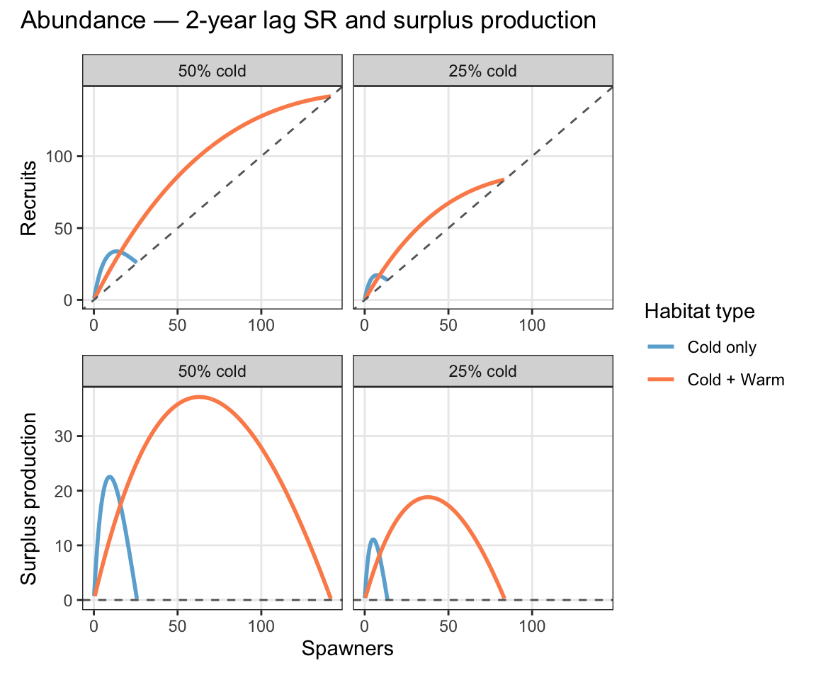
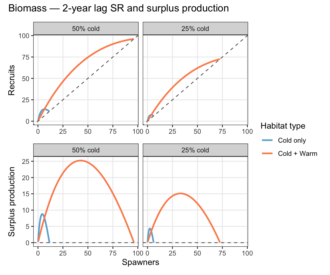
#### Compare representative SR relationships
```{r}
#| fig-width: 6
#| fig-height: 5
lag2curves <- bind_rows(
  sr_by_lag[[1]]$pred_b %>% mutate(measure = "biomass"),
  sr_by_lag[[1]]$pred_n %>% mutate(measure = "abundance"),
) %>%
  mutate(surplus = y - x) %>% filter(surplus > 0)

make_sr_plot <- function(m) {
  lag2curves %>% filter(measure == m) %>%
    ggplot(aes(x = x, y = y, color = hab_type)) +
    geom_line(linewidth = 1) +
    geom_abline(intercept = 0, slope = 1, linetype = "dashed", color = "grey40") +
    scale_color_manual(values = hab_cols, name = "Habitat type") +
    facet_wrap(~prop_cold_fact, nrow = 1) +
    labs(x = NULL, y = "Recruits") +
    theme_bw(base_size = 11) +
    theme(panel.grid.minor = element_blank())
}

make_sp_plot <- function(m) {
  lag2curves %>% filter(measure == m) %>%
    ggplot(aes(x = x, y = surplus, color = hab_type)) +
    geom_line(linewidth = 1) +
    geom_hline(yintercept = 0, linetype = "dashed", color = "grey40") +
    scale_color_manual(values = hab_cols, name = "Habitat type") +
    facet_wrap(~prop_cold_fact, nrow = 1) +
    labs(x = "Spawners", y = "Surplus production") +
    theme_bw(base_size = 11) +
    theme(panel.grid.minor = element_blank())
}

(make_sr_plot("abundance") / make_sp_plot("abundance")) +
  plot_layout(guides = "collect") +
  plot_annotation(title = "Abundance — 2-year lag SR and surplus production")
(make_sr_plot("biomass") / make_sp_plot("biomass")) +
  plot_layout(guides = "collect") +
  plot_annotation(title = "Biomass — 2-year lag SR and surplus production")
```
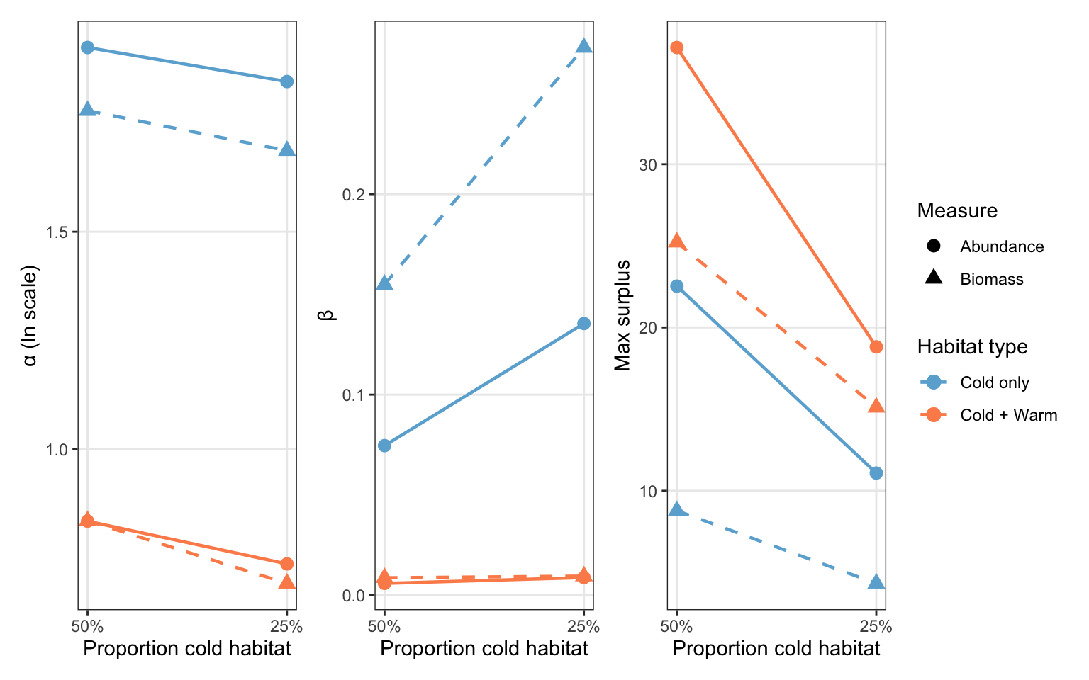
Ricker parameters (alpha, beta) and maximum surplus production from the 2-year lag fits, as a function of proportion cold habitat:
```{r}
#| fig-width: 8
#| fig-height: 5
# Extract Ricker parameters and max surplus from the 2-year lag hab_fits
ricker_params <- purrr::map_dfr(sr_by_lag[[1]]$hab_fits, \(hf) {
  tibble(
    hab_type       = hf$hab_type,
    prop_cold_fact = hf$prop_cold_fact,
    prop_cold      = as.numeric(sub("% cold", "", hf$prop_cold_fact)) / 100,
    alpha_n        = hf$alpha_n,
    beta_n         = hf$beta_n,
    max_surplus_n  = max(hf$pred_n$y - hf$pred_n$x),
    alpha_b        = hf$alpha_b,
    beta_b         = hf$beta_b,
    max_surplus_b  = max(hf$pred_b$y - hf$pred_b$x)
  )
}) |>
  mutate(hab_type = factor(hab_type, levels = c("Cold only", "Cold + Warm")))

pc_x <- scale_x_reverse(name = "Proportion cold habitat",
                        breaks = c(0.25, 0.50),
                        labels = scales::label_percent())

p_alpha <- ggplot(ricker_params, aes(x = prop_cold, color = hab_type, group = hab_type)) +
  geom_line(aes(y = alpha_n), linewidth = 0.8, linetype = "solid") +
  geom_point(aes(y = alpha_n, shape = "Abundance"), size = 3) +
  geom_line(aes(y = alpha_b), linewidth = 0.8, linetype = "dashed") +
  geom_point(aes(y = alpha_b, shape = "Biomass"), size = 3) +
  scale_color_manual(values = hab_cols, name = "Habitat type") +
  scale_shape_manual(values = c("Abundance" = 16, "Biomass" = 17), name = "Measure") +
  pc_x +
  labs(y = "\u03b1 (ln scale)") +
  theme_bw(base_size = 11) +
  theme(panel.grid.minor = element_blank())

p_beta <- ggplot(ricker_params, aes(x = prop_cold, color = hab_type, group = hab_type)) +
  geom_line(aes(y = beta_n), linewidth = 0.8, linetype = "solid") +
  geom_point(aes(y = beta_n, shape = "Abundance"), size = 3) +
  geom_line(aes(y = beta_b), linewidth = 0.8, linetype = "dashed") +
  geom_point(aes(y = beta_b, shape = "Biomass"), size = 3) +
  scale_color_manual(values = hab_cols, name = "Habitat type") +
  scale_shape_manual(values = c("Abundance" = 16, "Biomass" = 17), name = "Measure") +
  pc_x +
  labs(y = "\u03b2") +
  theme_bw(base_size = 11) +
  theme(panel.grid.minor = element_blank())

p_maxsurp <- ggplot(ricker_params, aes(x = prop_cold, color = hab_type, group = hab_type)) +
  geom_line(aes(y = max_surplus_n), linewidth = 0.8, linetype = "solid") +
  geom_point(aes(y = max_surplus_n, shape = "Abundance"), size = 3) +
  geom_line(aes(y = max_surplus_b), linewidth = 0.8, linetype = "dashed") +
  geom_point(aes(y = max_surplus_b, shape = "Biomass"), size = 3) +
  scale_color_manual(values = hab_cols, name = "Habitat type") +
  scale_shape_manual(values = c("Abundance" = 16, "Biomass" = 17), name = "Measure") +
  pc_x +
  labs(y = "Max surplus") +
  theme_bw(base_size = 11) +
  theme(panel.grid.minor = element_blank())

(p_alpha + p_beta + p_maxsurp) +
  plot_layout(guides = "collect") &
  theme(legend.position = "right")
```
#### Surplus production vs. harvest rate
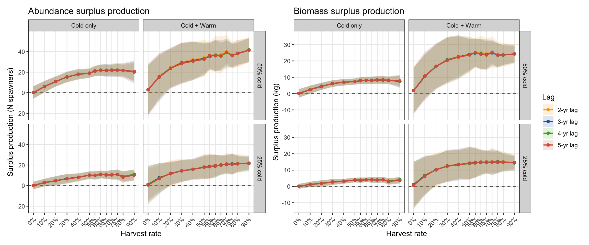
Surplus production per year is the signed distance above the 1:1 line: recruited adults minus the parent spawning stock. Positive = net gain; zero = replacement; negative = decline.
```{r}
#| fig-width: 12
#| fig-height: 5
# Annual SP = recruited adults(Y) minus parent spawners(Y - lag)
sp_ts <- purrr::map_dfr(sr_by_lag, \(x) {
  x$ts |>
    mutate(sp_n = n_recruited    - n_spawners_parent,
           sp_b = biom_recruited - biom_spawners_parent,
           lag  = factor(x$lag, levels = 2:5, labels = c("2-yr lag", "3-yr lag", "4-yr lag", "5-yr lag")),
           prod = log(n_recruited / n_spawners_parent))
})

sp_summ <- sp_ts |>
  group_by(lag, hab_type, prop_cold, prop_cold_fact, harvest_rate, harvest_rate_fact) |>
  summarise(
    n_spawn_mean = mean(n_spawners), n_spawn_sd = sd(n_spawners),
    b_spawn_mean = mean(biom_spawners), b_spawn_sd = sd(biom_spawners),
    sp_n_mean = mean(sp_n), sp_n_sd = sd(sp_n),
    sp_b_mean = mean(sp_b), sp_b_sd = sd(sp_b),
    prod_mean = mean(prod), prod_sd = sd(prod),
    .groups = "drop"
  )

lag_pal <- c("2-yr lag" = "orange", "3-yr lag" = "#2166AC", "4-yr lag" = "#4DAC26", "5-yr lag" = "#D6604D")

sp_base <- ggplot(sp_summ, aes(x = harvest_rate, color = lag, fill = lag)) +
  geom_hline(yintercept = 0, linetype = "dashed", color = "grey40") +
  scale_color_manual(values = lag_pal, name = "Lag") +
  scale_fill_manual( values = lag_pal, name = "Lag") +
  scale_x_continuous(breaks = hr_levels_mech,
                     labels = hr_labels_mech,
                     name   = "Harvest rate") +
  theme_bw(base_size = 11) +
  facet_grid(prop_cold_fact ~ hab_type) +
  theme(panel.grid.minor = element_blank(),
        axis.text.x = element_text(angle = 45, hjust = 1),
        legend.position = "none")

p_sp_n <- sp_base +
  geom_ribbon(aes(ymin = sp_n_mean - sp_n_sd,
                  ymax = sp_n_mean + sp_n_sd),
              alpha = 0.15, color = NA) +
  geom_line(aes(y = sp_n_mean), linewidth = 0.8) +
  geom_point(aes(y = sp_n_mean), size = 2, shape = 16) +
  labs(y = "Surplus production (N spawners)",
       title = "Abundance surplus production")

p_sp_b <- sp_base +
  geom_ribbon(aes(ymin = sp_b_mean - sp_b_sd,
                  ymax = sp_b_mean + sp_b_sd),
              alpha = 0.15, color = NA) +
  geom_line(aes(y = sp_b_mean), linewidth = 0.8) +
  geom_point(aes(y = sp_b_mean), size = 2, shape = 16) +
  labs(y = "Surplus production (kg)",
       title = "Biomass surplus production")

p_sp_n + p_sp_b +
  plot_layout(guides = "collect") &
  theme(legend.position = "right")
```
*These plots almost exactly match the harvest summary plots above, which show mean abundance and biomass of the harvest across harvest/exploitation rates. This makes sense: surplus is simply the harvestable biomass.*
Inspect relationships between productivity (logged recruits per spawner) and harvest rate and spawning stock biomass.
```{r}
#| fig-width: 7
#| fig-height: 8
p1 <- sp_ts %>% filter(lag == "2-yr lag") %>%
  ggplot(aes(x = jitter(harvest_rate), y = prod, color = harvest_rate_fact)) +
  geom_hline(yintercept = 0, linetype = "dashed") +
  geom_point(alpha = 0.25, size = 1.5, shape = 16) +
  geom_point(data = sp_summ %>% filter(lag == "3-yr lag"),
             inherit.aes = FALSE, size = 3,
             aes(x = harvest_rate, y = prod_mean, color = harvest_rate_fact)) +
  geom_errorbar(data = sp_summ %>% filter(lag == "3-yr lag"),
                inherit.aes = FALSE,
                aes(x = harvest_rate, ymin = prod_mean - prod_sd, ymax = prod_mean + prod_sd, color = harvest_rate_fact),
                width = 0, linewidth = 0.5) +
  scale_color_manual(values = hr_pal, name = "Harvest rate") +
  facet_grid(prop_cold_fact ~ hab_type) +
  labs(x = "Harvest rate", y = "Productivity, ln(R/S)") +
  theme_bw(base_size = 11) +
  theme(panel.grid.minor = element_blank(), legend.position = "none")


p2 <- ggplot() +
  geom_hline(yintercept = 0, linetype = "dashed") +
  geom_point(data = sp_ts %>% filter(lag == "3-yr lag"),
             aes(x = biom_spawners, y = prod, color = harvest_rate_fact),
             alpha = 0.25, size = 1.5, shape = 16) +
  geom_point(data = sp_summ %>% filter(lag == "3-yr lag"),
             inherit.aes = FALSE, size = 3,
             aes(x = b_spawn_mean, y = prod_mean, color = harvest_rate_fact)) +
  geom_errorbar(data = sp_summ %>% filter(lag == "3-yr lag"),
                inherit.aes = FALSE,
                aes(x = b_spawn_mean, ymin = prod_mean - prod_sd, ymax = prod_mean + prod_sd, color = harvest_rate_fact),
                width = 0, linewidth = 0.5) +
  geom_segment(data = sp_summ %>% filter(lag == "3-yr lag"),
               inherit.aes = FALSE,
               aes(x = b_spawn_mean - b_spawn_sd, xend = b_spawn_mean + b_spawn_sd,
                   y = prod_mean, yend = prod_mean,
                   color = harvest_rate_fact)) +
  scale_color_manual(values = hr_pal, name = "Harvest rate") +
  facet_grid(prop_cold_fact ~ hab_type) +
  labs(x = "Spawning stock biomass (kg)", y = "Productivity, ln(R/S)") +
  theme_bw(base_size = 11) +
  theme(panel.grid.minor = element_blank(), legend.position = "none")

(p1 / p2) +
  # plot_layout(guides = "collect") &
  theme(legend.position = "right")
```
### Total-adult based
Stock is defined as all adults (>200 g) present at the October 1 census in year Y−lag, with no harvest correction. Recruits are the total adults in the October 1 census of year Y plus fish harvested in summer of year Y (those removed before the census who would otherwise have been counted). Unlike the spawner-based approach, this definition includes adults that did not spawn due to poor condition, capturing condition-driven variation in spawning propensity across habitat scenarios and cold proportions.
#### Derive stock-recruitment curves
Derive adult-to-adult stock-recruitment curves over 4 different lag periods (2–5 years), for abundance and biomass separately.
```{r}
#| fig-width: 14
#| fig-height: 18
# ── Total adult abundance and biomass per scenario per year ───────────────────
# Stock  (X): Oct 1 census adults > 200 g only — no harvest correction
# Recruits (Y): Oct 1 census adults + same-year harvest (removed before census)
get_total_adults <- function(scen) {
  base_cols <- list(
    hab_type          = scen$ht,
    prop_cold         = scen$pc,
    prop_cold_fact    = factor(
      pc_labels_mech[match(scen$pc, pc_levels_mech)],
      levels = pc_labels_mech
    ),
    harvest_rate      = scen$hr,
    harvest_rate_fact = factor(scen$hr,
                               levels = hr_levels_mech,
                               labels = hr_labels_mech)
  )
  oct_adults <- scen$oct1_exp |>
    filter(peak_weight > 200) |>
    group_by(yr) |>
    summarise(n_oct1    = n(),
              biom_oct1 = sum(weight) / 1000,   # g -> kg
              .groups   = "drop")

  if (is.null(scen$harvest)) {
    oct_adults |>
      right_join(sr_exp_years, by = "yr") |>
      replace_na(list(n_oct1 = 0L, biom_oct1 = 0)) |>
      mutate(n_harv = 0L, biom_harv = 0,
             n_total_adults    = n_oct1,
             biom_total_adults = biom_oct1,
             !!!base_cols,
             hab_type = factor(hab_type, levels = c("Cold only", "Cold + Warm")))
  } else {
    harv_yr <- scen$harvest |>
      group_by(yr = year) |>
      summarise(n_harv    = n(),
                biom_harv = sum(weight) / 1000,
                .groups   = "drop")
    oct_adults |>
      right_join(sr_exp_years, by = "yr") |>
      left_join(harv_yr, by = "yr") |>
      replace_na(list(n_oct1 = 0L, biom_oct1 = 0, n_harv = 0L, biom_harv = 0)) |>
      mutate(n_total_adults    = n_oct1    + n_harv,
             biom_total_adults = biom_oct1 + biom_harv,
             !!!base_cols) |>
      mutate(hab_type = factor(hab_type, levels = c("Cold only", "Cold + Warm")))
  }
}

total_adults_ts <- purrr::map_dfr(ibm_list_mech, get_total_adults)

# ── Build lagged SR dataset + Ricker fits ────────────────────────────────────
build_adult_sr_v2 <- function(lag) {
  ts <- total_adults_ts |>
    select(hab_type, prop_cold, prop_cold_fact, harvest_rate, harvest_rate_fact,
           yr, n_recruited = n_total_adults, biom_recruited = biom_total_adults) |>
    mutate(yr_parent = yr - lag) |>
    left_join(
      total_adults_ts |>
        transmute(hab_type, prop_cold, yr, harvest_rate,
                  n_stock    = n_oct1,
                  biom_stock = biom_oct1),
      by = c("hab_type", "prop_cold", "yr_parent" = "yr", "harvest_rate")
    ) |>
    filter(!is.na(n_stock), n_stock > 0, n_recruited > 0) |>
    mutate(hab_type = factor(hab_type, levels = c("Cold only", "Cold + Warm")))

  summ <- ts |>
    group_by(hab_type, prop_cold, prop_cold_fact, harvest_rate, harvest_rate_fact) |>
    summarise(
      across(c(n_recruited, n_stock, biom_recruited, biom_stock),
             list(mean = mean, sd = sd)),
      .groups = "drop"
    )

  # Fit Ricker separately per hab_type × prop_cold group
  hab_fits <- ts |>
    group_by(hab_type, prop_cold, prop_cold_fact) |>
    group_split() |>
    purrr::map(\(d) {
      fit_n <- tryCatch(
        nls(n_recruited ~ a * n_stock * exp(-b * n_stock),
            data = d, start = list(a = 5, b = 0.05)),
        error = \(e) NULL)
      fit_b <- tryCatch(
        nls(biom_recruited ~ a * biom_stock * exp(-b * biom_stock),
            data = d, start = list(a = 5, b = 0.05)),
        error = \(e) NULL)
      N_seq <- seq(0, max(d$n_stock),    length.out = 300)
      B_seq <- seq(0, max(d$biom_stock), length.out = 300)
      mk_pred <- function(fit, xvar, seq_) {
        if (is.null(fit)) return(
          tibble(x = numeric(), y = numeric(),
                 hab_type = character(), prop_cold_fact = character()))
        tibble(x = seq_,
               y = predict(fit, setNames(list(seq_), xvar)),
               hab_type       = d$hab_type[1],
               prop_cold_fact = d$prop_cold_fact[1])
      }
      list(
        hab_type       = as.character(d$hab_type[1]),
        prop_cold_fact = as.character(d$prop_cold_fact[1]),
        alpha_n  = if (!is.null(fit_n)) log(coef(fit_n)["a"]) else NA,
        alpha_b  = if (!is.null(fit_b)) log(coef(fit_b)["a"]) else NA,
        beta_n   = if (!is.null(fit_n)) coef(fit_n)["b"]      else NA,
        beta_b   = if (!is.null(fit_b)) coef(fit_b)["b"]      else NA,
        s_star_n = if (!is.null(fit_n)) log(coef(fit_n)["a"]) / coef(fit_n)["b"] else NA,
        s_star_b = if (!is.null(fit_b)) log(coef(fit_b)["a"]) / coef(fit_b)["b"] else NA,
        pred_n   = mk_pred(fit_n, "n_stock",    N_seq),
        pred_b   = mk_pred(fit_b, "biom_stock", B_seq)
      )
    })

  # Combine predictions, preserving hab_type and prop_cold_fact for faceting
  pred_n <- purrr::map_dfr(hab_fits, "pred_n") |>
    mutate(hab_type = factor(hab_type, levels = c("Cold only", "Cold + Warm")))
  pred_b <- purrr::map_dfr(hab_fits, "pred_b") |>
    mutate(hab_type = factor(hab_type, levels = c("Cold only", "Cold + Warm")))

  list(lag = lag, ts = ts, summ = summ, hab_fits = hab_fits,
       pred_n = pred_n, pred_b = pred_b)
}

sr_v2 <- purrr::map(2:5, build_adult_sr_v2)

# Print equilibrium S* for each lag × hab_type × prop_cold
purrr::walk(sr_v2, \(x)
  purrr::walk(x$hab_fits, \(hf)
    cat(sprintf("Lag %d yr [%s, %s] — S* abundance: %.1f | S* biomass: %.2f kg\n",
                x$lag, hf$hab_type, hf$prop_cold_fact,
                hf$s_star_n %||% NA, hf$s_star_b %||% NA))
  )
)
# ── Helper: one adult SR panel ────────────────────────────────────────────────
adult_sr_panel_v2 <- function(dat, summ, x_raw, y_raw, x_summ, y_summ,
                               x_sd, y_sd, pred_df, x_lab, y_lab, title) {
  ggplot(dat, aes(x = {{ x_raw }}, y = {{ y_raw }}, color = harvest_rate_fact)) +
    geom_abline(slope = 1, intercept = 0,
                color = "grey50", linewidth = 0.5, linetype = "dashed") +
    geom_point(alpha = 0.2, size = 1.5, shape = 16) +
    geom_point(data = summ, inherit.aes = FALSE,
               aes(x = {{ x_summ }}, y = {{ y_summ }},
                   color = harvest_rate_fact),
               size = 3.5, shape = 16) +
    geom_errorbar(data = summ, inherit.aes = FALSE,
                  aes(x    = {{ x_summ }},
                      ymin = pmax(0, {{ y_summ }} - {{ y_sd }}),
                      ymax = {{ y_summ }} + {{ y_sd }},
                      color = harvest_rate_fact),
                  width = 0, linewidth = 0.5) +
    geom_segment(data = summ, inherit.aes = FALSE,
                 aes(x    = pmax(0, {{ x_summ }} - {{ x_sd }}),
                     xend = {{ x_summ }} + {{ x_sd }},
                     y    = {{ y_summ }}, yend = {{ y_summ }},
                     color = harvest_rate_fact),
                 linewidth = 0.5) +
    geom_line(data = pred_df, inherit.aes = FALSE,
              aes(x = x, y = y),
              linewidth = 0.5, color = "black") +
    scale_color_manual(values = hr_pal, name = "Harvest rate") +
    scale_x_continuous(labels = scales::label_comma()) +
    scale_y_continuous(labels = scales::label_comma()) +
    expand_limits(x = 0, y = 0) +
    facet_wrap(~ prop_cold_fact + hab_type, nrow = 2, scales = "free") +
    labs(x = x_lab, y = y_lab, title = title) +
    theme_bw(base_size = 11) +
    theme(panel.grid.minor = element_blank(), legend.position = "none")
}

# ── Build all panels (4 lags × 2 metrics) and assemble ───────────────────────
panels_v2 <- purrr::map(sr_v2, \(x) {
  list(
    n = adult_sr_panel_v2(
      dat = x$ts, summ = x$summ,
      x_raw  = n_stock,      y_raw  = n_recruited,
      x_summ = n_stock_mean, y_summ = n_recruited_mean,
      x_sd   = n_stock_sd,   y_sd   = n_recruited_sd,
      pred_df = x$pred_n,
      x_lab = glue::glue("Total adults (N), Oct 1 year Y\u2212{x$lag}"),
      y_lab = "Total adults (N), Oct 1(Y) + harvest(Y)",
      title = glue::glue("{x$lag}-yr lag (abundance)")
    ),
    b = adult_sr_panel_v2(
      dat = x$ts, summ = x$summ,
      x_raw  = biom_stock,      y_raw  = biom_recruited,
      x_summ = biom_stock_mean, y_summ = biom_recruited_mean,
      x_sd   = biom_stock_sd,   y_sd   = biom_recruited_sd,
      pred_df = x$pred_b,
      x_lab = glue::glue("Total adults (kg), Oct 1 year Y\u2212{x$lag}"),
      y_lab = "Total adults (kg), Oct 1(Y) + harvest(Y)",
      title = glue::glue("{x$lag}-yr lag (biomass)")
    )
  )
})

(panels_v2[[1]]$n + panels_v2[[1]]$b) /
(panels_v2[[2]]$n + panels_v2[[2]]$b) /
(panels_v2[[3]]$n + panels_v2[[3]]$b) /
(panels_v2[[4]]$n + panels_v2[[4]]$b) +
  plot_layout(guides = "collect") &
  theme(legend.position = "right")
```
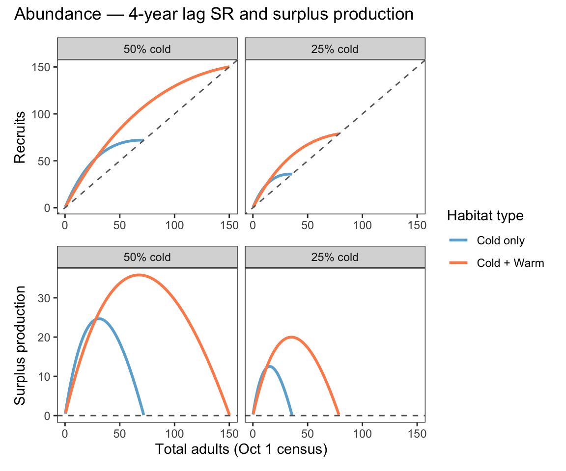
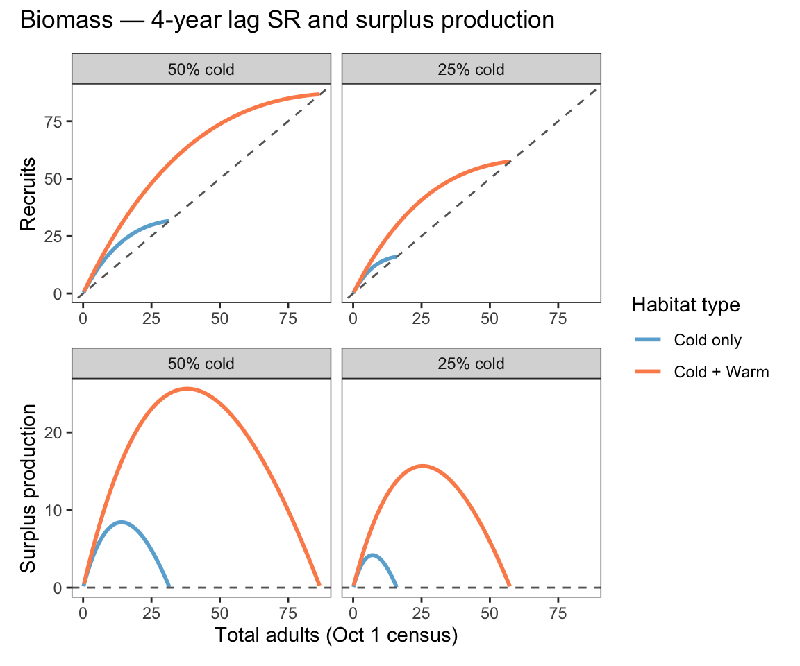
#### Compare representative SR relationships
```{r}
#| fig-width: 6
#| fig-height: 5
lag2curves_v2 <- bind_rows(
  sr_v2[[3]]$pred_b |> mutate(measure = "biomass"),
  sr_v2[[3]]$pred_n |> mutate(measure = "abundance")
) |>
  mutate(surplus = y - x) |>
  filter(surplus > 0)

make_sr_plot_v2 <- function(m) {
  lag2curves_v2 |> filter(measure == m) |>
    ggplot(aes(x = x, y = y, color = hab_type)) +
    geom_line(linewidth = 1) +
    geom_abline(intercept = 0, slope = 1, linetype = "dashed", color = "grey40") +
    scale_color_manual(values = hab_cols, name = "Habitat type") +
    facet_wrap(~prop_cold_fact, nrow = 1) +
    labs(x = NULL, y = "Recruits") +
    theme_bw(base_size = 11) +
    theme(panel.grid = element_blank())
}

make_sp_plot_v2 <- function(m) {
  lag2curves_v2 |> filter(measure == m) |>
    ggplot(aes(x = x, y = surplus, color = hab_type)) +
    geom_line(linewidth = 1) +
    geom_hline(yintercept = 0, linetype = "dashed", color = "grey40") +
    scale_color_manual(values = hab_cols, name = "Habitat type") +
    facet_wrap(~prop_cold_fact, nrow = 1) +
    labs(x = "Total adults (Oct 1 census)", y = "Surplus production") +
    theme_bw(base_size = 11) +
    theme(panel.grid = element_blank())
}

(make_sr_plot_v2("abundance") / make_sp_plot_v2("abundance")) +
  plot_layout(guides = "collect") +
  plot_annotation(title = "Abundance \u2014 4-year lag SR and surplus production")
(make_sr_plot_v2("biomass") / make_sp_plot_v2("biomass")) +
  plot_layout(guides = "collect") +
  plot_annotation(title = "Biomass \u2014 4-year lag SR and surplus production")
```
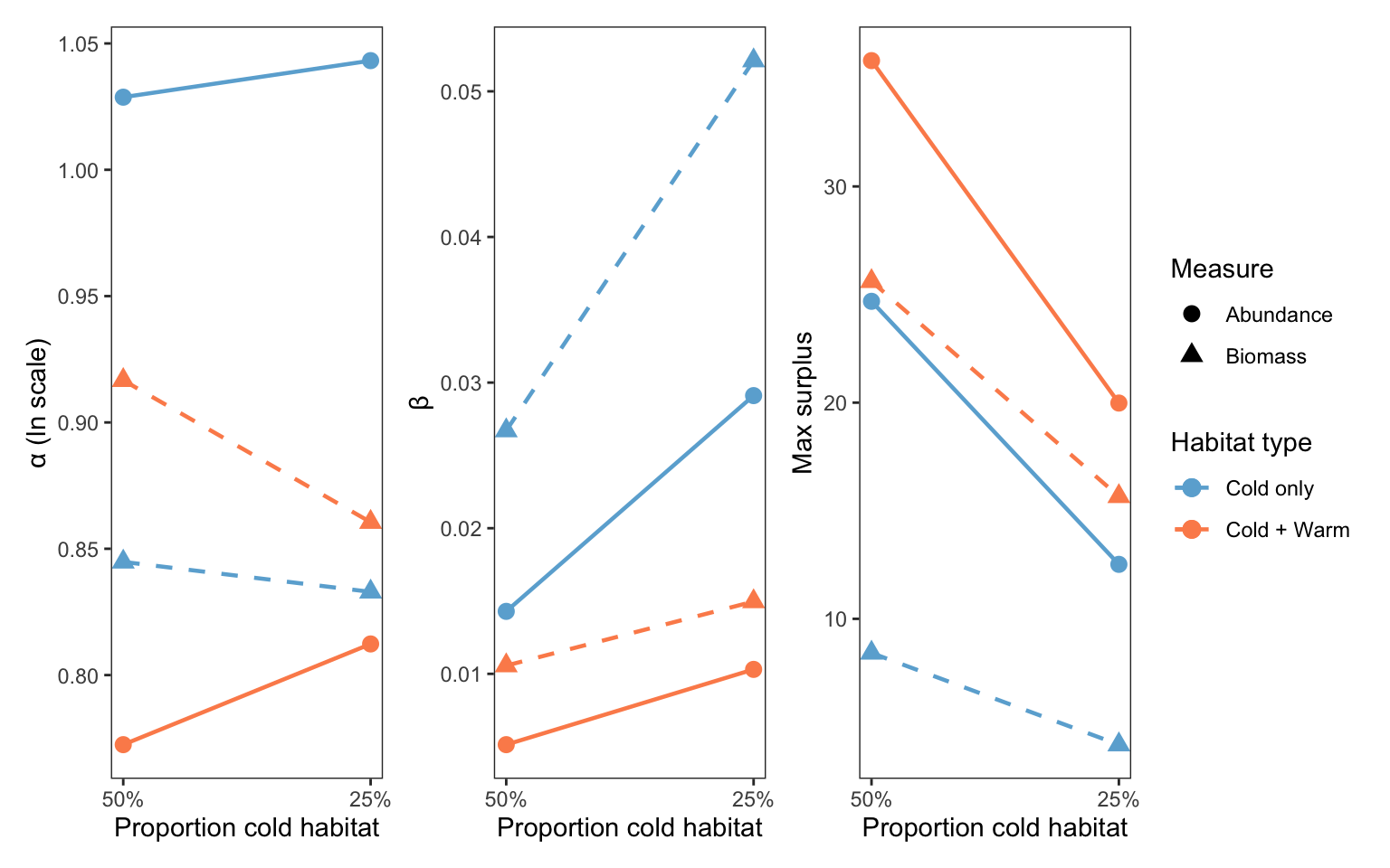
Ricker parameters (alpha, beta) and maximum surplus production from the 4-year lag fits, as a function of proportion cold habitat:
```{r}
#| fig-width: 8
#| fig-height: 5
ricker_params_ta <- purrr::map_dfr(sr_v2[[3]]$hab_fits, \(hf) {
  tibble(
    hab_type       = hf$hab_type,
    prop_cold_fact = hf$prop_cold_fact,
    prop_cold      = as.numeric(sub("% cold", "", hf$prop_cold_fact)) / 100,
    alpha_n        = hf$alpha_n,
    beta_n         = hf$beta_n,
    max_surplus_n  = max(hf$pred_n$y - hf$pred_n$x),
    alpha_b        = hf$alpha_b,
    beta_b         = hf$beta_b,
    max_surplus_b  = max(hf$pred_b$y - hf$pred_b$x)
  )
}) |>
  mutate(hab_type = factor(hab_type, levels = c("Cold only", "Cold + Warm")))

p_alpha_ta <- ggplot(ricker_params_ta,
                     aes(x = prop_cold, color = hab_type, group = hab_type)) +
  geom_line(aes(y = alpha_n), linewidth = 0.8, linetype = "solid") +
  geom_point(aes(y = alpha_n, shape = "Abundance"), size = 3) +
  geom_line(aes(y = alpha_b), linewidth = 0.8, linetype = "dashed") +
  geom_point(aes(y = alpha_b, shape = "Biomass"), size = 3) +
  scale_color_manual(values = hab_cols, name = "Habitat type") +
  scale_shape_manual(values = c("Abundance" = 16, "Biomass" = 17), name = "Measure") +
  pc_x +
  labs(y = "\u03b1 (ln scale)") +
  theme_bw(base_size = 11) +
  theme(panel.grid = element_blank())

p_beta_ta <- ggplot(ricker_params_ta,
                    aes(x = prop_cold, color = hab_type, group = hab_type)) +
  geom_line(aes(y = beta_n), linewidth = 0.8, linetype = "solid") +
  geom_point(aes(y = beta_n, shape = "Abundance"), size = 3) +
  geom_line(aes(y = beta_b), linewidth = 0.8, linetype = "dashed") +
  geom_point(aes(y = beta_b, shape = "Biomass"), size = 3) +
  scale_color_manual(values = hab_cols, name = "Habitat type") +
  scale_shape_manual(values = c("Abundance" = 16, "Biomass" = 17), name = "Measure") +
  pc_x +
  labs(y = "\u03b2") +
  theme_bw(base_size = 11) +
  theme(panel.grid = element_blank())

p_maxsurp_ta <- ggplot(ricker_params_ta,
                       aes(x = prop_cold, color = hab_type, group = hab_type)) +
  geom_line(aes(y = max_surplus_n), linewidth = 0.8, linetype = "solid") +
  geom_point(aes(y = max_surplus_n, shape = "Abundance"), size = 3) +
  geom_line(aes(y = max_surplus_b), linewidth = 0.8, linetype = "dashed") +
  geom_point(aes(y = max_surplus_b, shape = "Biomass"), size = 3) +
  scale_color_manual(values = hab_cols, name = "Habitat type") +
  scale_shape_manual(values = c("Abundance" = 16, "Biomass" = 17), name = "Measure") +
  pc_x +
  labs(y = "Max surplus") +
  theme_bw(base_size = 11) +
  theme(panel.grid = element_blank())

(p_alpha_ta + p_beta_ta + p_maxsurp_ta) +
  plot_layout(guides = "collect") &
  theme(legend.position = "right")
```
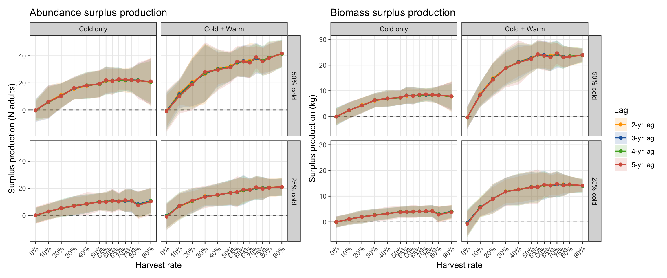
#### Surplus production vs. harvest rate
Surplus production per year is the signed distance above the 1:1 line: total recruited adults (Oct 1 census + same-year harvest) minus the total adult stock in year Y−lag. Positive = net gain; zero = replacement; negative = decline.
```{r}
#| fig-width: 12
#| fig-height: 5
sp_ts_ta <- purrr::map_dfr(sr_v2, \(x) {
  x$ts |>
    mutate(sp_n = n_recruited - n_stock,
           sp_b = biom_recruited - biom_stock,
           lag  = factor(x$lag, levels = 2:5,
                         labels = c("2-yr lag", "3-yr lag", "4-yr lag", "5-yr lag")),
           prod = log(n_recruited / n_stock))
})

sp_summ_ta <- sp_ts_ta |>
  group_by(lag, hab_type, prop_cold, prop_cold_fact, harvest_rate, harvest_rate_fact) |>
  summarise(
    n_stock_mean    = mean(n_stock),    n_stock_sd    = sd(n_stock),
    biom_stock_mean = mean(biom_stock), biom_stock_sd = sd(biom_stock),
    sp_n_mean = mean(sp_n), sp_n_sd = sd(sp_n),
    sp_b_mean = mean(sp_b), sp_b_sd = sd(sp_b),
    prod_mean = mean(prod), prod_sd  = sd(prod),
    .groups = "drop"
  )

sp_base_ta <- ggplot(sp_summ_ta, aes(x = harvest_rate, color = lag, fill = lag)) +
  geom_hline(yintercept = 0, linetype = "dashed", color = "grey40") +
  scale_color_manual(values = lag_pal, name = "Lag") +
  scale_fill_manual( values = lag_pal, name = "Lag") +
  scale_x_continuous(breaks = hr_levels_mech,
                     labels = hr_labels_mech,
                     name   = "Harvest rate") +
  theme_bw(base_size = 11) +
  facet_grid(prop_cold_fact ~ hab_type) +
  theme(panel.grid.minor = element_blank(),
        axis.text.x = element_text(angle = 45, hjust = 1),
        legend.position = "none")

p_sp_n_ta <- sp_base_ta +
  geom_ribbon(aes(ymin = sp_n_mean - sp_n_sd,
                  ymax = sp_n_mean + sp_n_sd),
              alpha = 0.15, color = NA) +
  geom_line(aes(y  = sp_n_mean), linewidth = 0.8) +
  geom_point(aes(y = sp_n_mean), size = 2, shape = 16) +
  labs(y = "Surplus production (N adults)",
       title = "Abundance surplus production")

p_sp_b_ta <- sp_base_ta +
  geom_ribbon(aes(ymin = sp_b_mean - sp_b_sd,
                  ymax = sp_b_mean + sp_b_sd),
              alpha = 0.15, color = NA) +
  geom_line(aes(y  = sp_b_mean), linewidth = 0.8) +
  geom_point(aes(y = sp_b_mean), size = 2, shape = 16) +
  labs(y = "Surplus production (kg)",
       title = "Biomass surplus production")

p_sp_n_ta + p_sp_b_ta +
  plot_layout(guides = "collect") &
  theme(legend.position = "right")
```
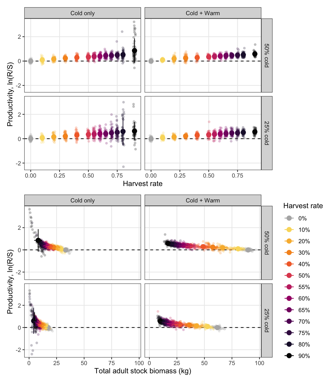
Inspect relationships between productivity (logged recruits per total adult stock) and harvest rate and stock biomass.
```{r}
#| fig-width: 7
#| fig-height: 8
p1_ta <- sp_ts_ta |> filter(lag == "4-yr lag") |>
  ggplot(aes(x = jitter(harvest_rate), y = prod, color = harvest_rate_fact)) +
  geom_hline(yintercept = 0, linetype = "dashed") +
  geom_point(alpha = 0.25, size = 1.5, shape = 16) +
  geom_point(data = sp_summ_ta |> filter(lag == "2-yr lag"),
             inherit.aes = FALSE, size = 3,
             aes(x = harvest_rate, y = prod_mean, color = harvest_rate_fact)) +
  geom_errorbar(data = sp_summ_ta |> filter(lag == "2-yr lag"),
                inherit.aes = FALSE,
                aes(x = harvest_rate,
                    ymin = prod_mean - prod_sd,
                    ymax = prod_mean + prod_sd,
                    color = harvest_rate_fact),
                width = 0, linewidth = 0.5) +
  scale_color_manual(values = hr_pal, name = "Harvest rate") +
  facet_grid(prop_cold_fact ~ hab_type) +
  labs(x = "Harvest rate", y = "Productivity, ln(R/S)") +
  theme_bw(base_size = 11) +
  theme(panel.grid.minor = element_blank(), legend.position = "none")

p2_ta <- ggplot() +
  geom_hline(yintercept = 0, linetype = "dashed") +
  geom_point(data = sp_ts_ta |> filter(lag == "2-yr lag"),
             aes(x = biom_stock, y = prod, color = harvest_rate_fact),
             alpha = 0.25, size = 1.5, shape = 16) +
  geom_point(data = sp_summ_ta |> filter(lag == "2-yr lag"),
             inherit.aes = FALSE, size = 3,
             aes(x = biom_stock_mean, y = prod_mean, color = harvest_rate_fact)) +
  geom_errorbar(data = sp_summ_ta |> filter(lag == "2-yr lag"),
                inherit.aes = FALSE,
                aes(x    = biom_stock_mean,
                    ymin  = prod_mean - prod_sd,
                    ymax  = prod_mean + prod_sd,
                    color = harvest_rate_fact),
                width = 0, linewidth = 0.5) +
  geom_segment(data = sp_summ_ta |> filter(lag == "2-yr lag"),
               inherit.aes = FALSE,
               aes(x    = biom_stock_mean - biom_stock_sd,
                   xend = biom_stock_mean + biom_stock_sd,
                   y    = prod_mean, yend = prod_mean,
                   color = harvest_rate_fact)) +
  scale_color_manual(values = hr_pal, name = "Harvest rate") +
  facet_grid(prop_cold_fact ~ hab_type) +
  labs(x = "Total adult stock biomass (kg)", y = "Productivity, ln(R/S)") +
  theme_bw(base_size = 11) +
  theme(panel.grid.minor = element_blank(), legend.position = "none")

(p1_ta / p2_ta) +
  theme(legend.position = "right")
```
## Fry production vs. recruitment
Declining fry input with stable recruitment output demonstrates density-dependent compensation at the cold-habitat summer bottleneck. The gap between the two panels quantifies how much excess fry production the system can absorb before the bottleneck is breached.
```{r eval=FALSE}
#| cache: false
#| fig-width: 7
#| fig-height: 6
get_annual_fry <- function(scen) {
  scen$fry_annual |>
    right_join(all_exp_years, by = "yr") |>
    replace_na(list(n_fry = 0L)) |>
    mutate(harvest_rate = factor(scen$hr,
                                 levels = hr_levels_mech,
                                 labels = hr_labels_mech),
           hab_type = scen$ht)
}

fry_ts    <- purrr::map_dfr(ibm_list_mech, get_annual_fry) |>
  filter(hab_type == "Cold only")
age0_cold <- age0_ts |>
  filter(hab_type == "Cold only")

p_fry <- ggplot(fry_ts, aes(x = yr, y = n_fry, color = harvest_rate)) +
  geom_line(alpha = 0.25) +
  geom_smooth(linewidth = 0.8, se = FALSE) +
  scale_color_manual(values = hr_pal, guide = "none") +
  scale_x_continuous(name = NULL) +
  scale_y_continuous(name = "Annual fry production",
                     labels = scales::label_comma(),
                     limits = c(0, NA)) +
  theme_bw() +
  theme(panel.grid.minor = element_blank())

p_rec <- ggplot(age0_cold, aes(x = yr, y = n_age0, color = harvest_rate)) +
  geom_line(alpha = 0.25) +
  geom_smooth(linewidth = 0.8, se = FALSE) +
  scale_color_manual(values = hr_pal, name = "Harvest rate") +
  scale_x_continuous(name = "Year") +
  scale_y_continuous(name = "Age-0 recruits (Nov. 1)",
                     labels = scales::label_comma(),
                     limits = c(0, NA)) +
  theme_bw() +
  theme(panel.grid.minor = element_blank())

p_fry / p_rec + plot_layout(guides = "collect") & theme(legend.position = "right")
```